OH Utica Production, Water Usage, and Waste Disposal by County
Part II of a Multi-part Series
By Ted Auch, Great Lakes Program Coordinator, FracTracker Alliance

In this part of our ongoing “Water-Energy Nexus” series focusing on Water and Water Use, we are looking at how counties in Ohio differ between how much oil and gas are produced, as well as the amount of water used and waste produced. This analysis also highlights how the OH DNR’s initial Utica projections differ dramatically from the current state of affairs. In the first article in this series, we conducted an analysis of OH’s water-energy nexus showing that Utica wells are using an ave. of 5 million gallons/well. As lateral well lengths increase, so does water use. In this analysis we demonstrate that:

1. Drillers have to use more water, at higher pressures, to extract the same unit of oil or gas that they did years ago,
2. Where production is relatively high, water usage is lower,
3. As fracking operations move to the perimeter of a marginally productive play – and smaller LLCs and MLPs become a larger component of the landscape – operators are finding minimal returns on $6-8 million in well pad development costs,
4. Market forces and Muskingum Watershed Conservancy District (MWCD) policy has allowed industry to exploit OH’s freshwater resources at bargain basement prices relative to commonly agreed upon water pricing schemes.

At current prices¹, the shale gas industry is allocating < 0.27% of total well pad costs to current – and growing – freshwater requirements. It stands to reason that this multi-part series could be a jumping off point for a more holistic discussion of how we price our “endless” freshwater resources here in OH.

In an effort to better understand the inter-county differences in water usage, waste production, and hydrocarbon productivity across OH’s 19 Utica Shale counties we compiled a data-set for 500+ Utica wells which was previously used to look at differenced in these metrics across the state’s primary industry players. The results from Table 1 below are discussed in detail in the subsequent sections.

Table 1. Hydrocarbon production totals and per day values with top three producers in bold

Production

Total

It will come as no surprise to the reader that OH’s Utica oil and gas production is being led by Carroll County, followed distantly by Harrison, Noble, Belmont, Guernsey and Columbiana counties. Carroll has produced 3.7 million barrels of oil to date, while the latter have combined to produce an additional 4.5 million barrels. Carroll wells have been in production for nearly 67,000 days², while the aforementioned county wells have been producing for 42,886 days. The remaining counties are home to 49 wells that have been in production for nearly 8,800 days or 7% of total production days in Ohio.

Combined with the state’s remaining 49 producing wells spread across 13 counties, OH’s Utica Shale has produced 8.3 million barrels of oil as well as 251,844,311 Mcf³ of natural gas and 5.4 million barrels of brine. Oil and natural gas together have an estimated value of $2.99 billion ($213 million per quarter)⁴ assuming average oil and natural gas prices of $96 per barrel and $8.67 per Mcf during the current period of production (2011 to Q2-2014), respectively.

Potential Revenue at Different Severance Tax Rates:

• Current production tax, 0.5-0.8%: $19 million ($1.4 Million Per Quarter (MPQ). At this rate it would take the oil and gas industry 35 years to generate the $4.6 billion in tax revenue they proposed would be generated by 2020.
• Proposed, 1% gas and 4% oil: At Governor Kasich’s proposed tax rate, $2.99 billion translates into $54 million ($3.9 MPQ). It would still take 21 years to return the aforementioned $4.6 billion to the state’s coffers.
• Proposed, 5-7%: Even at the proposed rate of 5-7% by Policy Matters OH and northeastern OH Democrats, the industry would only have generated $179 million ($12.8 MPQ) to date. It would take 11 years to generate the remaining $4.42 billion in tax revenue promised by OH Oil and Gas Association’s (OOGA) partners at IHS “Energy Oil & Gas Industry Solutions” (NYSE: IHS).⁵

The bottom-line is that a production tax of 11-25% or more ($24-53 MPQ) would be necessary to generate the kind of tax revenue proposed by the end of 2020. This type of O&G taxation regime is employed in the states of Alaska and Oklahoma.

From an outreach and monitoring perspective, effects on air and water quality are two of the biggest gaps in our understanding of shale gas from a socioeconomic, health, and environmental perspective. Pulling out a mere 1% from any of these tax regimes would generate what we’ll call an “Environmental Monitoring Fee.” Available monitoring funds would range between $194,261 and $1.8 million ($16 million at 55%). These monies would be used to purchase 2-21 mobile air quality devices and 10-97 stream quantity/quality gauges to be deployed throughout the state’s primary shale counties to fill in the aforementioned data gaps.

Per-Day Production

On a per-day oil production basis, Belmont and Columbiana (20 barrels per day (BPD)) are overshadowed by Washington (59 BPD) and Muskingum (40 BPD) counties’ four giant Utica wells. Carroll is able to maintain such a high level of production relative to the other 15 counties by shear volume of producing wells; Noble (268 BPD), Guernsey (147 BPD), and Harrison (136 BPD) counties exceed Carroll’s production on a per-day basis. The bottom of the league table includes three oil-free wells in Ashland, Knox, and Medina, as well as seventeen <10 BPD wells in Jefferson and Mahoning counties.

With respect to natural gas, Harrison (1,840 Mcf per day (MPD)) and Guernsey counties are replaced by Monroe (7,348 MPD) and Jefferson (2,447 MPD) counties’ 26 Utica wells. The range of production rates for natural gas is represented by the king of natural gas producers, Belmont County, producing 8,578 MPD on the high end and Mahoning and Coshocton counties in addition to the aforementioned oil dry counties on the low end. Four of the five oil- or gas-dry counties produce the least amount of brine each day (BrPD). Coshocton, Medina, and Noble county Utica wells are currently generating 267-363 barrels of BrPD, with an additional seven counties generating 100-200 BrPD. Only four counties – 1.2% of OH Utica wells – are home to unconventional wells that generate ≤ 30 BrPD.

Water Usage

Freshwater is needed for the hydraulic fracturing process during well stimulation. For counties where we had compiled a respectable sample size we found that Monroe and Noble counties are home to the Utica wells requiring the greatest amount of freshwater to obtain acceptable levels of productivity (Figure 1). Monroe and Noble wells are using 10.6 and 8.8 million gallons (MGs) of water per well. Coshocton is home to a well that required 10.8 MGs, while Muskingum and Washington counties are home to wells that have utilized 10.2 and 9.5 MGs, respectively. Belmont, Guernsey, and Harrison reflect the current average state of freshwater usage by the Utica Shale industry in OH, with average requirements of 6.4, 6.9, and 7.2 MGs per well. Wells in eight other counties have used an average of 3.8 (Mahoning) to 5.4 MGs (Tuscarawas). The counties of Ashland, Knox, and Medina are home to wells requiring the least amount of freshwater in the range of 2.2-2.9 MGs. Overall freshwater demand on a per well basis is increasing by 220,500-333,300 gallons per quarter in Ohio with percent recycled water actually declining by 00.54% from an already trivial average of 6-7% in 2011 (Figure 2).

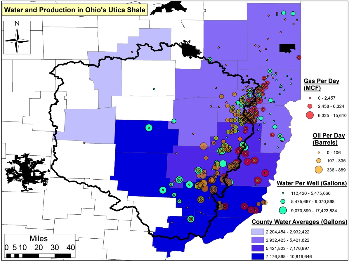Figure 1. Average water usage (gallons) per Utica well by county

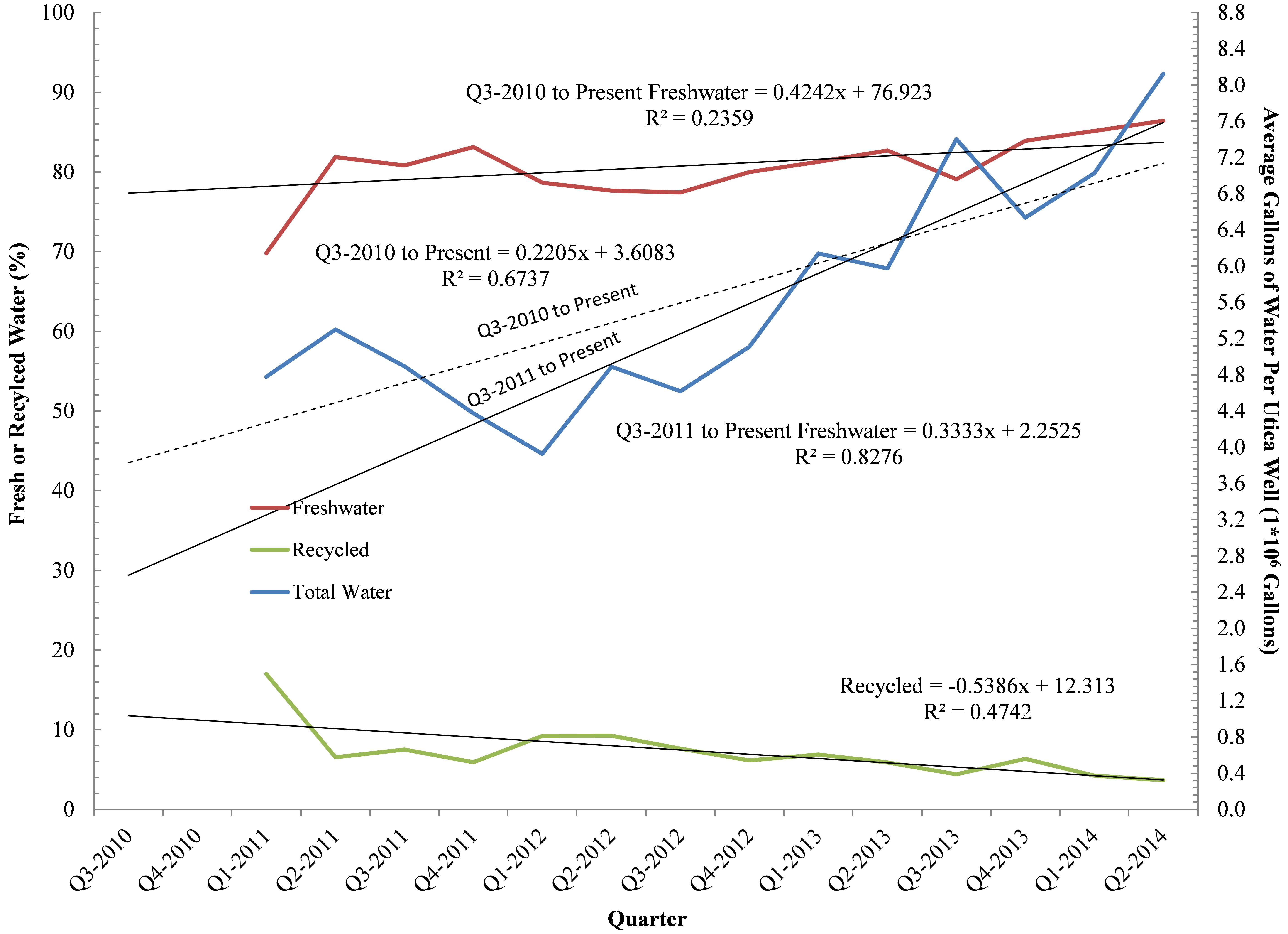Figure 2. Average water usage (gallons) on per well basis by OH Utica Shale industry, shown quarterly between Q3-2010 & Q2-2014.

Belmont County’s 30+ Utica wells are the least efficient with respect to oil recovery relative to freshwater requirements, averaging 7,190 gallons of water per gallon of oil (Figure 3). A distant second is Jefferson County’s 14 wells, which have required on average 3,205 gallons of water per gallon of oil. Columbiana’s 26 Utica wells are in third place requiring 1,093 gallons of freshwater. Coshocton, Mahoning, Monroe, and Portage counties are home to wells requiring 146-473 gallons for each gallon of oil produced.

Belmont County’s 14 Utica wells are the least efficient with respect to natural gas recovery relative to freshwater requirements (Figure 4). They average 1,306 gallons of water per Mcf. A distant second is Carroll County’s 250+ wells, which have injected 520 gallons of water 7,000+ feet below the earth’s service to produce a single Mcf of natural gas. Muskingum’s Utica well and Noble County’s 39 wells are the only other wells requiring more than 100 gallons of freshwater per Mcf. The remaining nine counties’ wells require 15-92 gallons of water to produce an Mcf of natural gas.

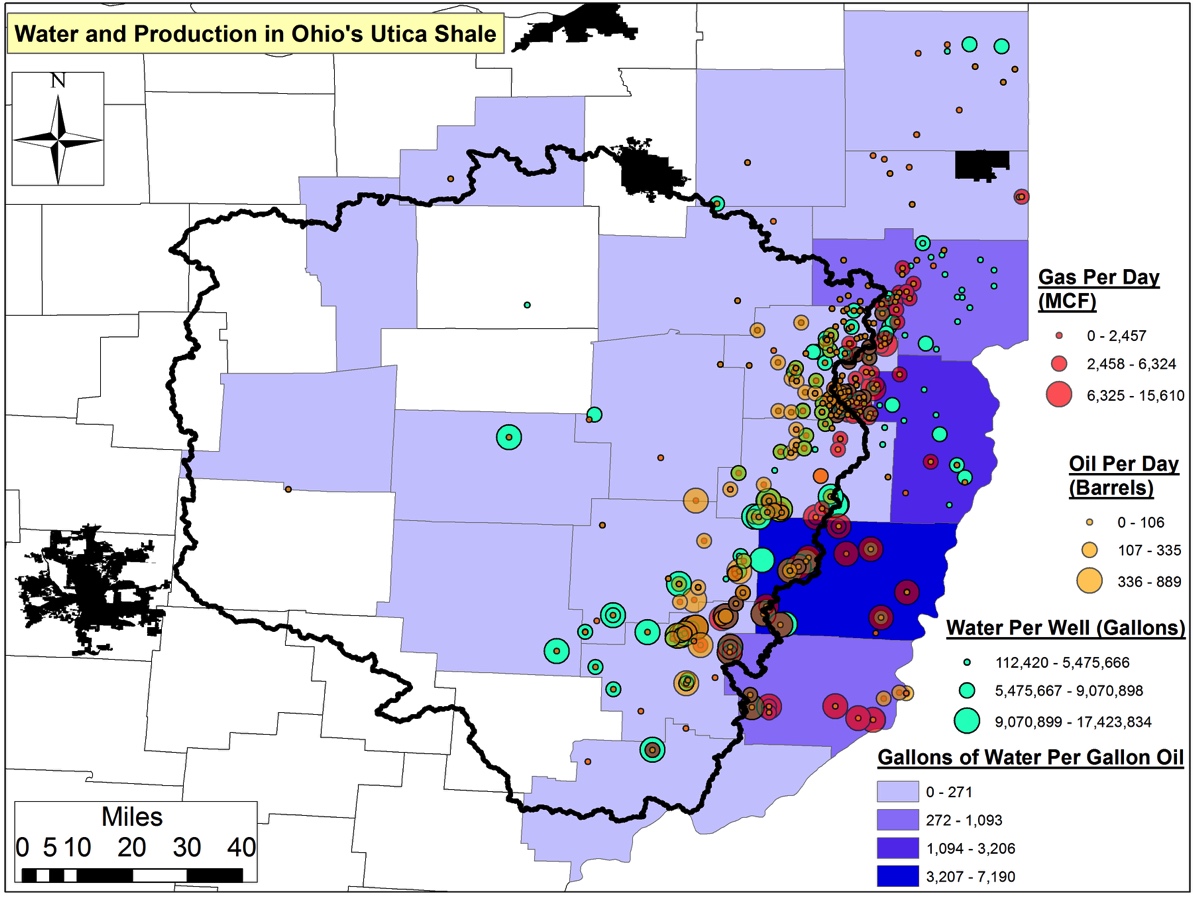Figure 3. Average water usage (gallons) per unit of oil (gallons) produced across 19 Ohio Utica counties

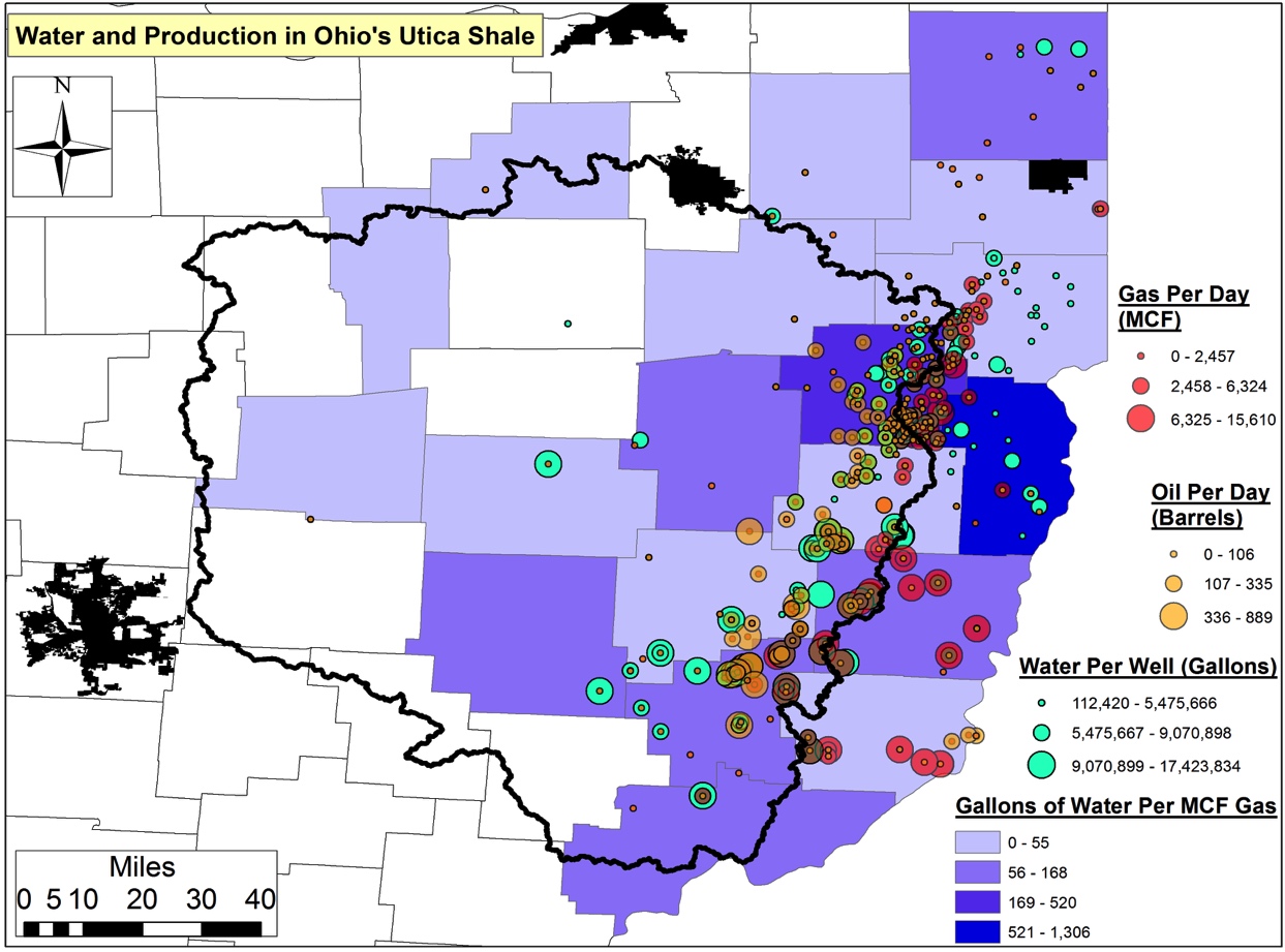Figure 4. Average water usage (gallons) per unit of gas produced (Mcf) across 19 Ohio Utica counties

Waste Production

The aforementioned Jefferson wells are the least efficient with respect to waste vs. product produced. Jefferson wells are generating 12,728 gallons of brine per gallon of oil (Figure 5).⁶ Wells from this county are followed distantly by the 32 Belmont and 26 Columbiana county wells, which are generating 5,830 and 3,976 gallons of brine per unit of oil.⁵ The remaining counties (for which we have data) are using 8-927 gallons of brine per unit of oil; six counties’ wells are generating <38 gallons of brine per gallon of oil.

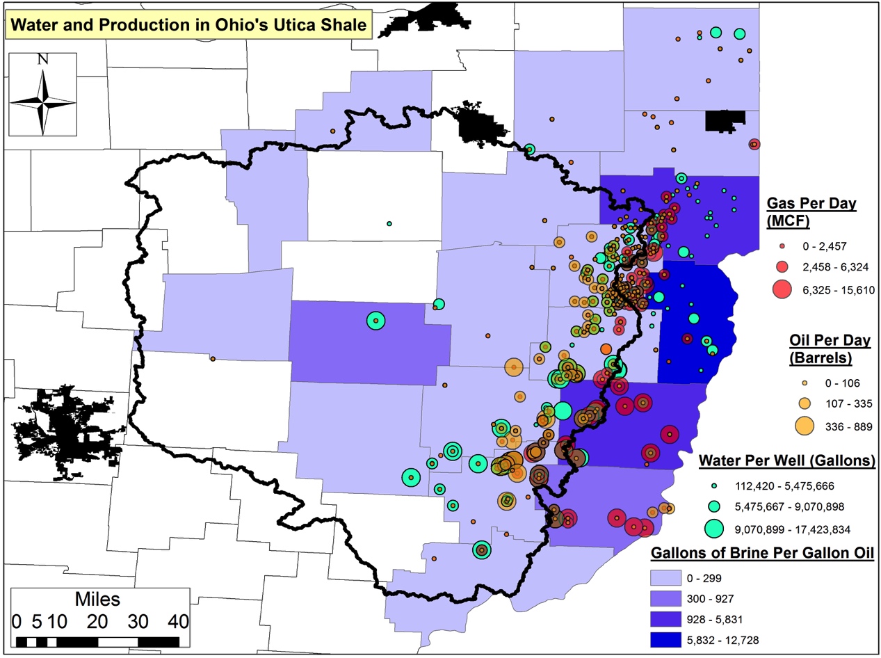
Figure 5. Average brine production (gallons) per gallon of oil produced per day across 19 Ohio Utica Counties

The average Utica well in OH is generating 820 gallons of fracking waste per unit of product produced. Across all OH Utica wells, an average of 0.078 gallons of brine is being generated for every gallon of freshwater used. This figure amounts to a current total of 233.9 MGs of brine waste produce statewide. Over the next five years this trend will result in the generation of one billion gallons (BGs) of brine waste and 12.8 BGs of freshwater required in OH. Put another way…

233.9 MGs is equivalent to the annual waste production of 5.2 million Ohioans – or 45% of the state’s current population. 

Due to the low costs incurred by industry when they choose to dispose of their fracking waste in OH, drillers will have only to incur $100 million over the next five years to pay for the injection of the above 1.0 BGs of brine. Ohioans, however, will pay at least $1.5 billion in the same time period to dispose of their municipal solid waste. The average fee to dispose of every ton of waste is $32, which means that the $100 million figure is at the very least $33.5 million – and as much as $250.6 million – less than we should expect industry should be paying to offset the costs.

Environmental Accounting

In summary, there are two ways to look at the potential “energy revolution” that is shale gas:

1. Using the same traditional supply-side economics metrics we have used in the past (e.g., globalization, Efficient Market Hypothesis, Trickle Down Economics, Bubbles Don’t Exist) to socialize long-term externalities and privatize short-term windfall profits, or
2. We can begin to incorporate into the national dialogue issues pertaining to watershed resilience, ecosystem services, and the more nuanced valuation of our ecosystems via Ecological Economics.

The latter will require a more real-time and granular understanding of water resource utilization and fracking waste production at the watershed and regional scale, especially as it relates to headline production and the often-trumpeted job generating numbers.

We hope to shed further light on this new “environmental accounting” as it relates to more thorough and responsible energy development policy at the state, federal, and global levels. The life cycle costs of shale gas drilling have all too often been ignored and can’t be if we are to generate the types of energy our country demands while also stewarding our ecosystems. As Mark Twain is reported to have said “Whiskey is for drinking; water is for fighting over.” In order to avoid such a battle over the water-energy nexus in the long run it is imperative that we price in the shale gas industry’s water-use footprint in the near term. As we have demonstrated so far with this series this issue is far from settled here in OH and as they say so goes Ohio so goes the nation!

A Moving Target

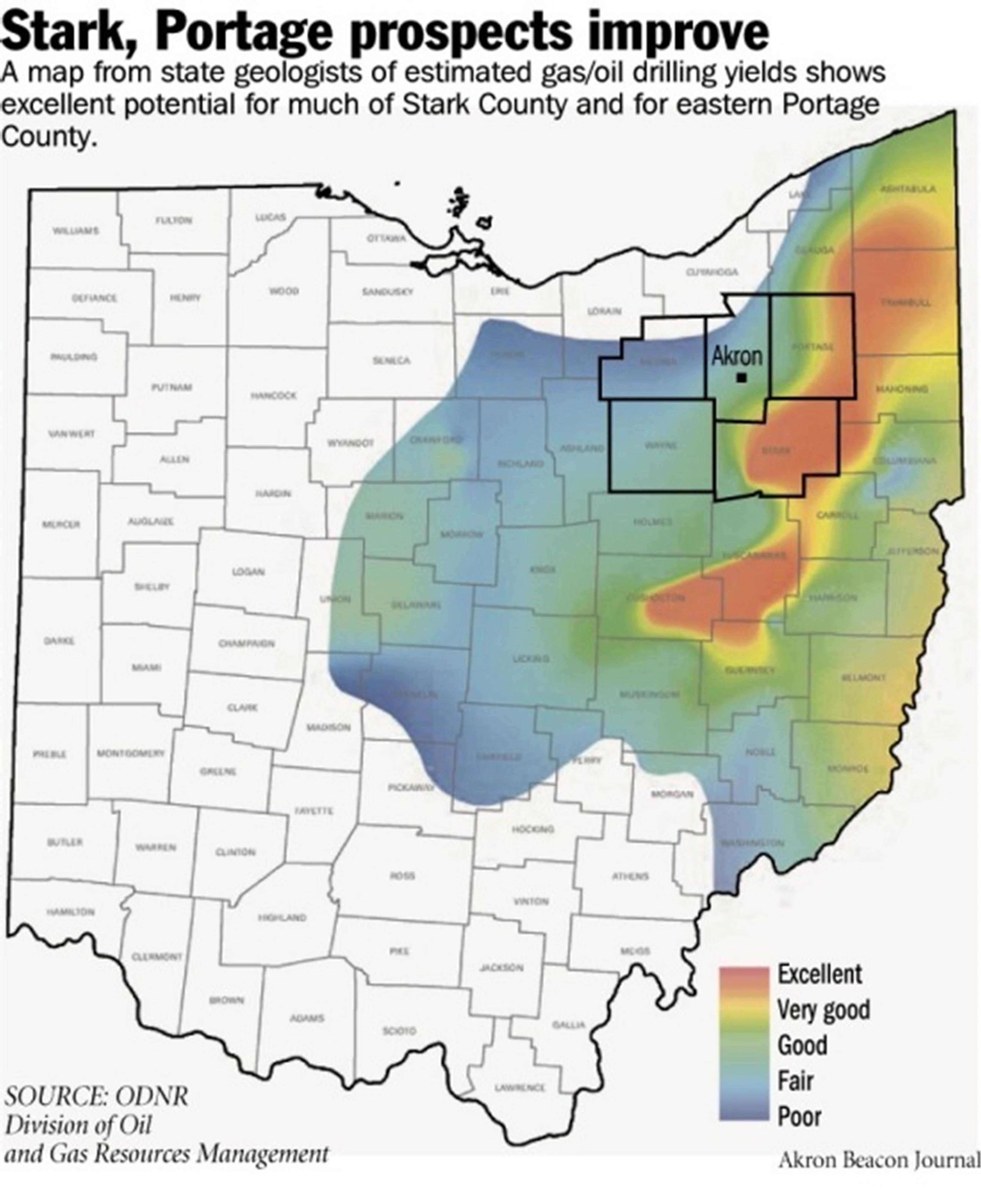
Figure 6. ODNR projection map of potential Utica productivity from spring 2012

OH’s Department of Natural Resources (ODNR) originally claimed a big red – and nearly continuous – blob of Utica productivity existed. The projection originally stretched from Ashtabula and Trumbull counties south-southwest to Tuscarawas, Guernsey, and Coshocton along the Appalachian Plateau (See Figure 6).

However, our analysis demonstrates that (Figures 7 and 8):

1. This is a rapidly moving target,
2. The big red blob isn’t as big – or continuous – as once projected, and
3. It might not even include many of the counties once thought to be the heart of the OH Utica shale play.

This last point is important because counties, families, investors, and outside interests were developing investment and/or savings strategies based on this map and a 30+ year timeframe – neither of which may be even remotely close according to our model.

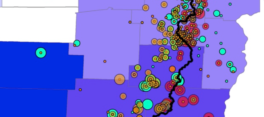
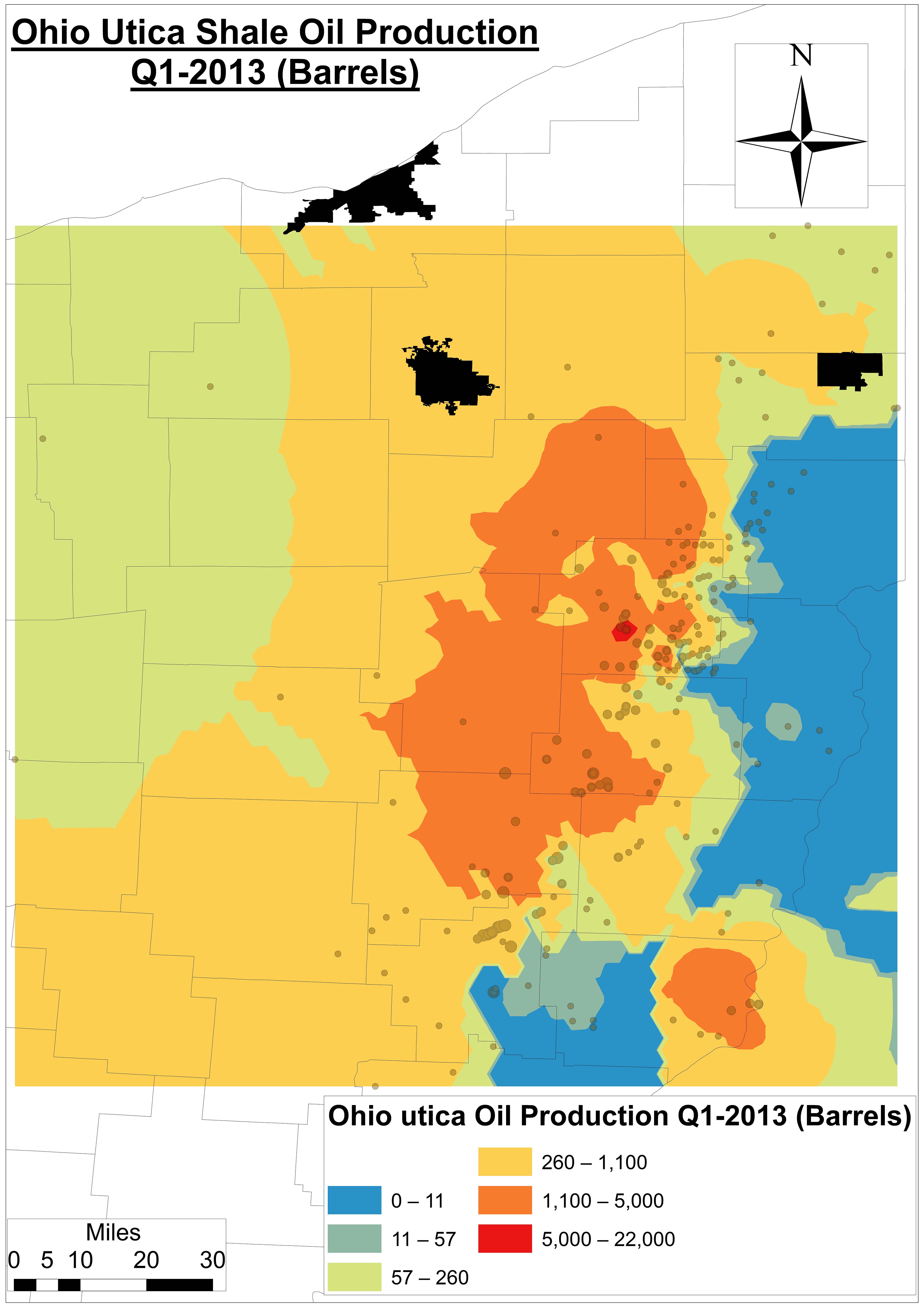Figure 7a. An Ohio Utica Shale oil production model using Kriging6 for Q1-2013	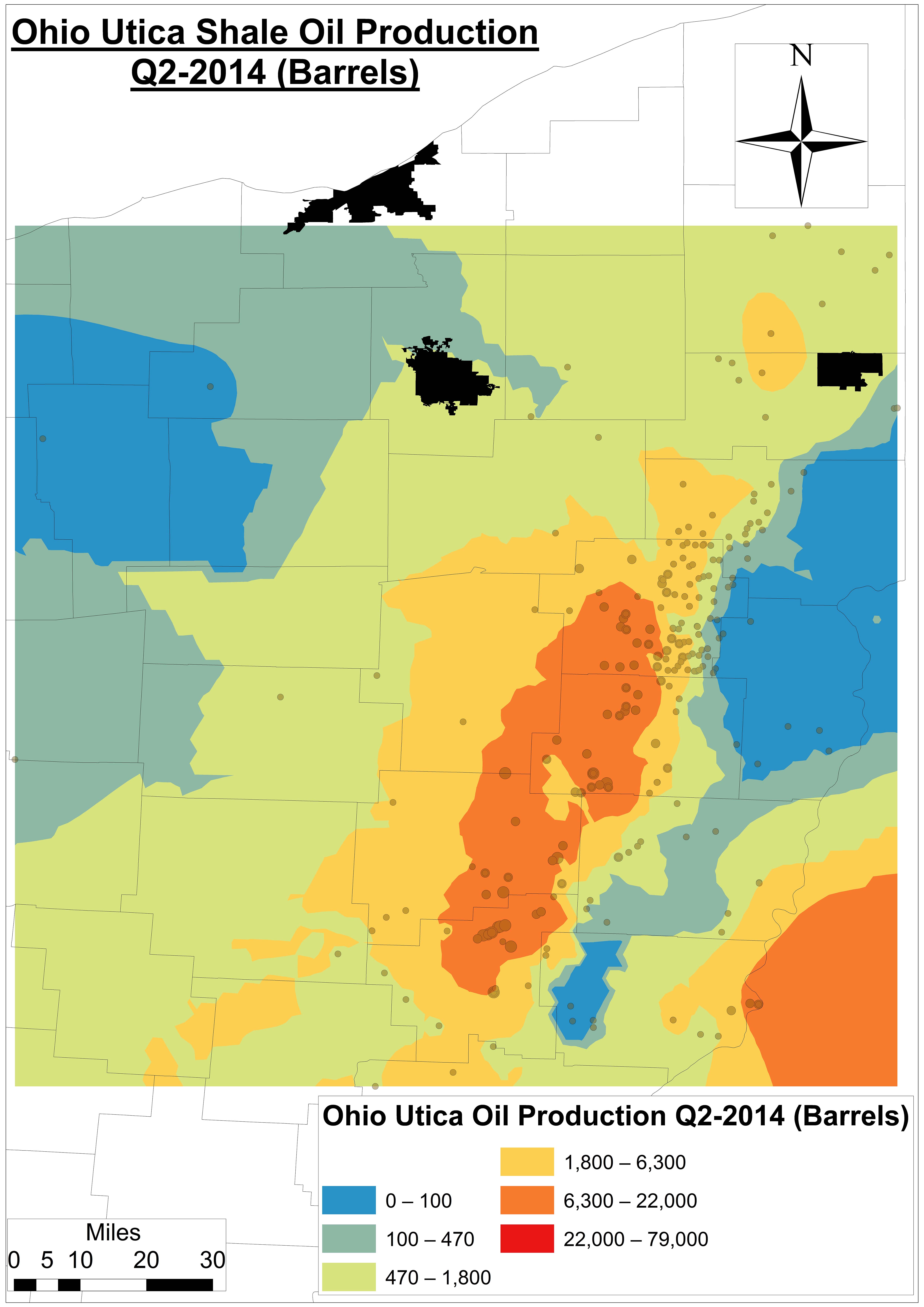Figure 7b. An Ohio Utica Shale oil production model using Kriging for Q2-2014
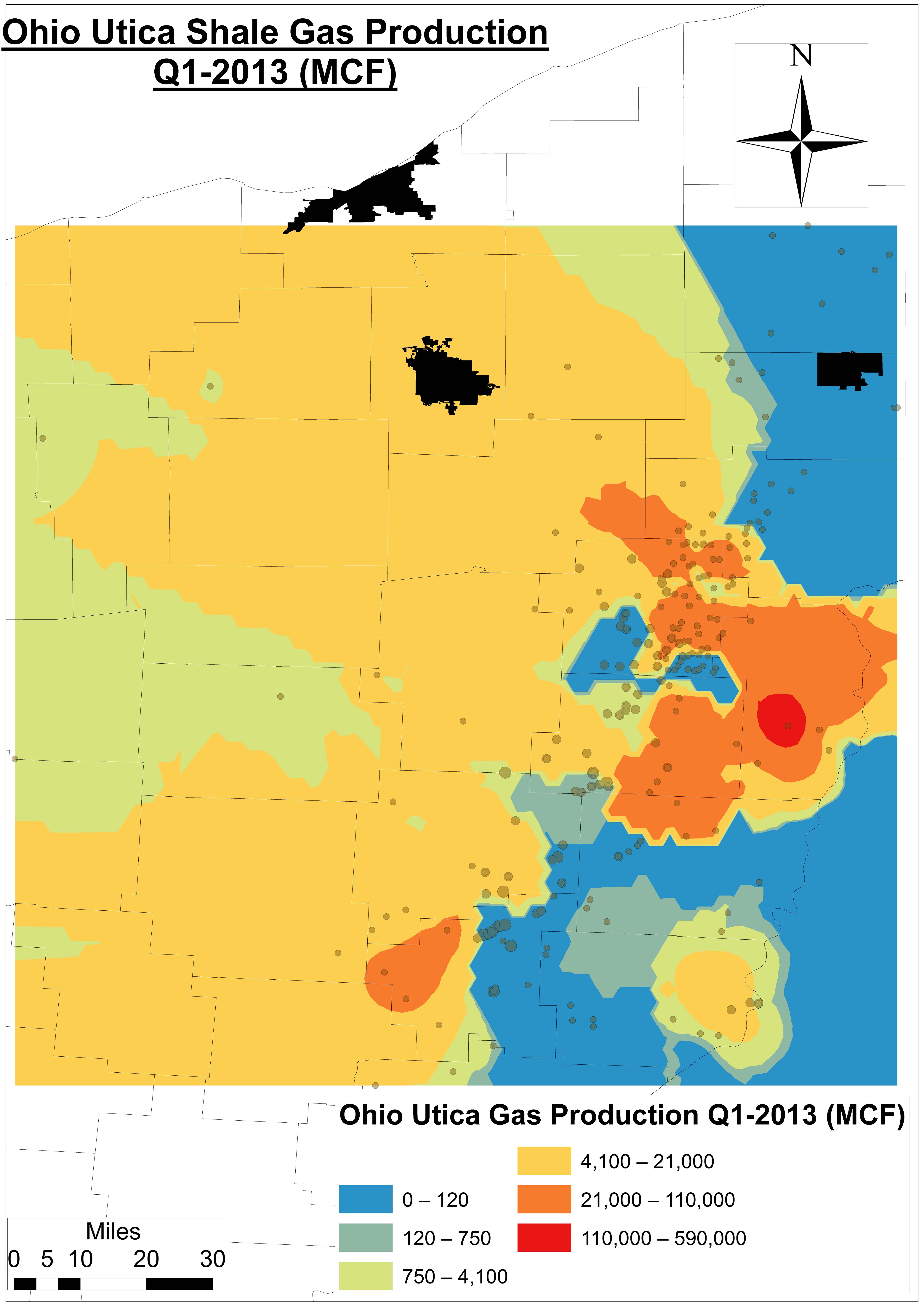Figure 8a. An Ohio Utica Shale gas production model using Kriging for Q1-2013	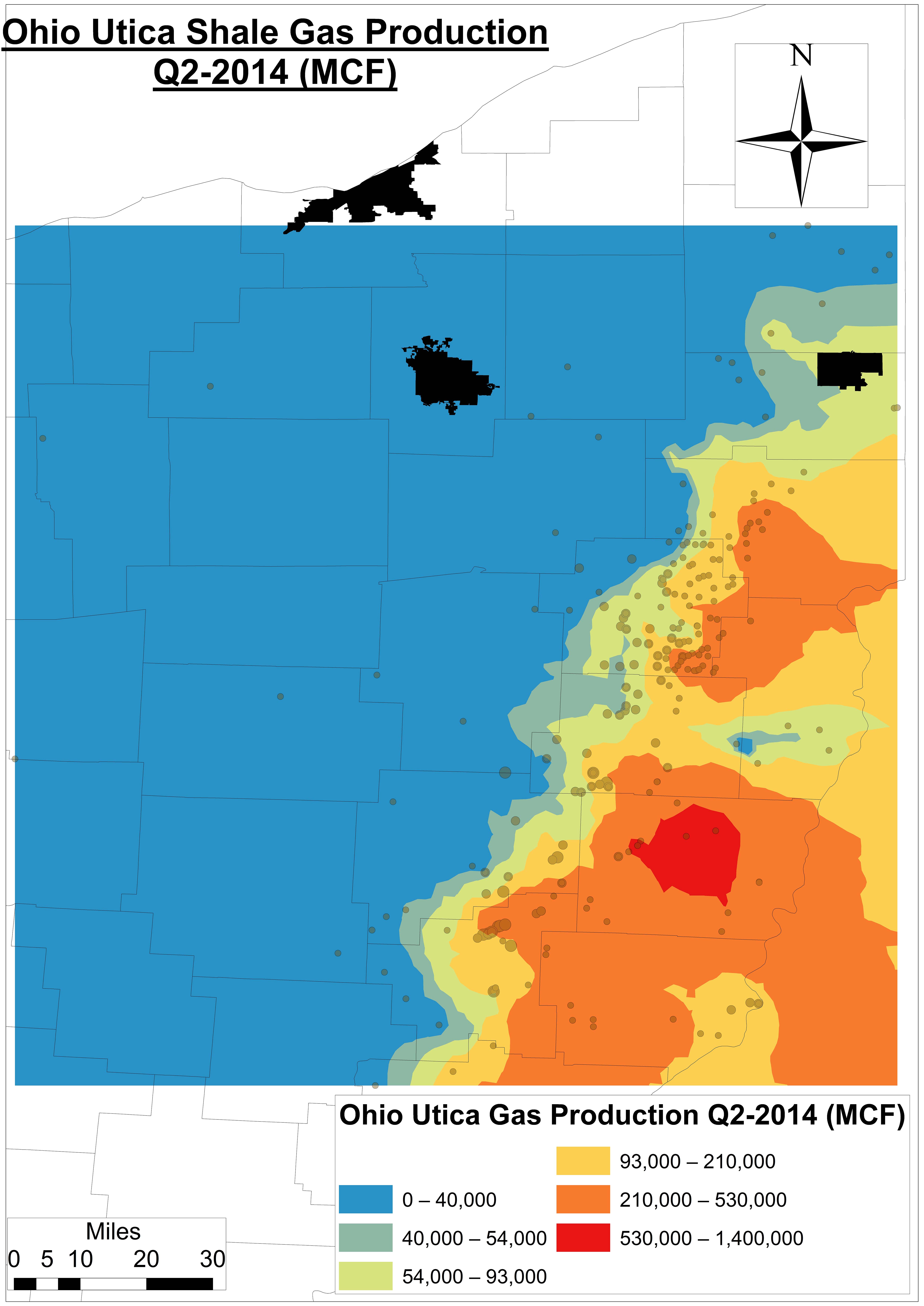Figure 8b. An Ohio Utica Shale gas production model using Kriging for Q2-2014

Footnotes

1. $4.25 per 1,000 gallons, which is the current going rate for freshwater at OH’s MWCD New Philadelphia headquarters, is 4.7-8.2 times less than residential water costs at the city level according to Global Water Intelligence.
2. Carroll County wells have seen days in production jump from 36-62 days in 2011-2012 to 68-78 in 2014 across 256 producing wells as of Q2-2014.
3. One Mcf is a unit of measurement for natural gas referring to 1,000 cubic feet, which is approximately enough gas to run an American household (e.g. heat, water heater, cooking) for four days.
4. Assuming average oil and natural gas prices of $96 per barrel and $8.67 per Mcf during the current period of production (2011 to Q2-2014), respectively
5. IHS’ share price has increased by $1.7 per month since publishing a report about the potential of US shale gas as a job creator and revenue generator
6. On a per-API# basis or even regional basis we have not found drilling muds data. We do have it – and are in the process of making sense of it – at the Solid Waste District level.
7. An interpolative Geostatistical technique formally called Empirical Bayesian Kriging.