Florida Hydraulic Fracturing, Proposed Drilling, and Seismic Tests

Over the last few months, we have received several requests to map drilling data in Florida. Below is the information we have been able to procure to-date.

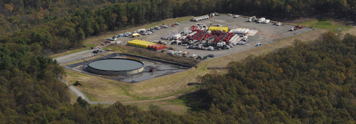
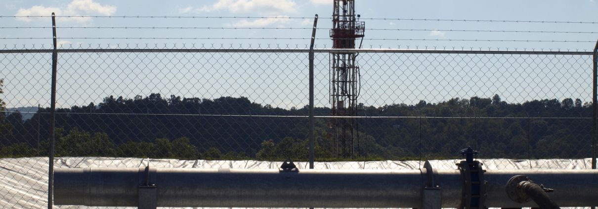
One of the newest controversies in the field of oil and gas extraction is playing out in South Florida, just outside of the City of Naples. While there has been history of oil and gas development, both on- and off-shore in Florida since the 1940s, the risks of fracturing rock to extract hydrocarbons more than 10,000 feet below the surface, has been gaining much attention recently.

The map below shows the locations of planned seismic testing for deep strata oil extraction in Collier and Hendry Counties, Florida, and also the location of a newly permitted exploratory oil well and an adjacent salt water injection well close to the center of the city of Naples, Florida, in the suburb of Golden Gate Estates. According to the final permit, filed 9/20/2013, the horizontally-drilled exploratory well, if it reaches “an economically viable layer and the applicant chooses to continue drilling operations…will proceed to a final depth of 16,600 feet measured depth/12,064 feet total vertical depth”. The nearby salt water injection well would be 2800 feet deep. This extraction targets a fossil fuel-bearing geological layer called the South Florida Basin Sunniland/Dollar Bay Basin. The method of extraction will be via “acid fracking” – the type of unconventional process proposed for the Monterey Shale in California – not hydraulic fracturing using water. Florida is underlain by limestone bedrock. Acid-fracking in this sort of geology creates cracks in the rock by dissolving the calcium carbonate, allowing trapped gas to escape.

In April 2013, in conjunction with the well permitting plan,  31 neighbors near the proposed well received notices that they were living in a “hydrogen sulfide evacuation zone.” Hydrogen sulfide is a often released from gas-bearing rock formations during drilling.

(Click here to be redirected to a full-screen version of this map, including a legend and capability to toggle layers on and off)

The drilling activities are being opposed by groups such as Preserve Our Paradise. Preserve Our Paradise was formed when residents learned that the Dan A. Hughes Company of Beeville, Texas had applied to drill a well that the organization feels presents threats to public safety and the natural environment. Members felt particular concern because the proposed well would be less than a mile from the “City of Naples main water wellfield, the future Collier County water wellfield area, the Florida Panther National Wildlife Preserve, and the residential suburb of Golden Gate Estates,” according to Preserve Our Paradise’s website. The Dan A. Hughes Company has already leased 115,000 environmentally sensitive acres of Southwest Florida for exploration. Two other petitions were filed opposing the well: one from the Stone Crab Alliance, a citizens’ group, and other by Matthew Schwartz, a Lake Worth resident. Both petitions cite concerns for panthers and other environmental issues.

Additional testing for oil and gas is may be occurring not far away. Companies, such as Kerogen Florida Operating Comp. LLC, Hendry Energy Services, and Tocala LLC have applied for permits to conduct seismic testing for oil in Hendry and Collier Counties, just north of Big Cypress National Preserve, according to the Florida Department of Environmental Protection’s Oil and Gas Drilling Applications Database.

EPA Region 4 will be holding a public hearing on the Golden Gate well permit, tentatively scheduled for February 27, 2014 at the Golden Gate Civic Association.

Addendum: In a victory for opponents of the drilling near the Panther refuge, Sierra Club reported that in mid July, 2014, the Dan Hughes Oil Company announced that it would be terminating its lease holdings on 115,000 acres in the area. Only a few weeks earlier, the Florida Department of Environmental Protection announced that the driller had been using illegal extraction techniques similar to fracking.

Data sources

Sustainability and Unconventional Drilling: Different Definitions, Shared Discourse

By Jill Terner, PA Communications Intern, FracTracker Alliance

In 1987, at the World Commission on Environment conference, sustainable development was recognized internationally for the first time. Sustainability in this sense is broadly defined as both the goal and process of serving present needs while not precluding the ability of future generations to serve their needs1. This general definition has lent itself well to becoming the cornerstone of arguments for and against drilling that uses hydraulic fracturing.

A largely economic definition of sustainability is behind many pro-drilling agendas, while environmental sustainability is mainly what informs regulatory or anti-drilling viewpoints2. Though these two parties make different uses of the term sustainability, they still share discourse on this topic. This common use that overlies differing connotations renders sustainability what Star & Griesemer (1989) would term a boundary object3.

Over the course of this blog series, I will look at how both industry and environmental regulatory committees are using the science at their disposal to make a case for or against unconventional drilling as a sustainable practice. Finally, I will finish by discussing how the shared discourse that uses these competing definitions impacts the court of public opinion.

Sustainability Defined by Industry

From an industrial perspective, sustainability is viewed in an economic light. Social, environmental, and other facets of sustainability aren’t ignored, though. Rather, they are seen as part of a cost-benefit equation wherein the potential impacts of industrial presence on communities and the environment are quantified and measured against the potential economic benefits associated with tapping into unconventional oil and gas reserves2,4.

The primary, direct economic benefit reported to be associated with this industry’s presence in communities is job creation. Industry leaders espouse the notion that allowing drilling in an area opens up job opportunities for rig workers. Extractive industries are typically located in economically depressed, non-metropolitan areas6. Thus, the benefit of employment and inferred family support is a great touted advantage4.

Additional direct benefits are associated with leasing of both land and mineral rights to grant drilling access to industry. Selling the mineral rights below a plot of land can be a lucrative option for those who own them. However, the mineral rights owners are not always the same people as those who own the land above the minerals to be leased. As such, landowners must be mindful of what is going on with the minerals beneath their property.

Ancillary businesses may also reap economic benefits associated with industry. Primarily, businesses that supply the materials needed in the construction and maintenance of the drilling operation can potentially benefit from industry presence. More indirectly, unrelated businesses such as hotels and restaurants in the community may stand to benefit from the influx of wealth associated with residents’ newfound employment.

These direct and indirect economic consequences are commonly viewed as a positive investment in the community by industry, and the local political leaders that support industry’s presence. If residents allow drilling, industry claims, they are making an investment towards economic stability and sustainability – which will be propagated by the influx of wealth due to job creation. Negative environmental and social impacts that may occur alongside this economic boon typically fall short of outweighing its benefits in the eyes of the industry.

How Industry Makes Use of Current Research

At present, there is relatively little scientific research done on the impacts of unconventional drilling. What research does exist on the sustainable impacts of unconventional drilling consists largely of studies funded by industry4. As hydraulic fracturing is a relatively new practice, more research continues to burgeon and inform questions regarding economic, social, and environmental impacts from all angles.

One way industry gets around the lack of pre-existing research is to do input-output analysis4. This analysis links the primary industry with ancillary ones through tables of coefficients, and calculates the estimated direct and indirect economic impacts through calculations using that table. While some of the calculated benefits may be viewed positively across the board, public perception of these gains may be different in different locations5, making it tough to generalize acceptance of findings.

Relatedly, industry also takes research done on the economic benefits incurred by communities and states where unconventional drilling has been in place longer, and applies the methods or results to areas where drilling is new4. For example, coefficients generated from an input-output equation from a Texas community could be used to project benefits for a community in New York. Analogy can be a powerful tool, and with the lack of research on current industrial practices, it is the best tool to use in certain circumstances. However, as geographic, economic, social, and environmental contingencies are different between locations of drilling, comparison may be somewhat limited.

Additionally, many pro-industry groups are dedicated to refuting scientific studies that have been put out by academics, environmental regulatory bodies, or independent researchers. For example, the website Energy in Depth published a thorough critique of the HBO documentary Gasland, debunking it point-by-point. When scientific research cannot be entirely disproved, promoting the benefits of unconventional drilling over the costs of another dirtier fuel, like coal, is also another way to promote drilling. While these cost-benefit-analyses can be legitimate, they often fail to incorporate the use and potential benefits of other energy resources, like wind.

What’s Next?

In the next installment of this series, I will discuss how regulatory committees are defining sustainability, and how they are mobilizing science towards their definition.


References

1. Dernbach, J. C., & Bernstein, S. (2003). Pursuing sustainable communities: Looking back, looking forward. The Urban Lawyer, 35(3), 495-532.

2. Finewood, M. H., & Stroup, L. J. (2012). Fracking and the neoliberalization of the hyrdo-social cycle in Pennsylvania’s Marcellus shale. Journal of Contemporary Water Research and Education, (147), 72-79.

3. Star, S. L., & Griesemer, J. R. (1989). Institutional ecology, ‘translations’ and boundary objects: Amateurs and professionals in Berkeley’s museum of vertebrate zoology, 1907-39. Social Studies of Science, 19, 387-420.

4. Barth, J. M. (2013). The economic impact of shale gas development on state and local economies: Benefits, costs, and uncertainties. New Solutions, 23(1), 85-101.

5. Perkins, N. D. (2012). The fracturing of place: The regulation of Marcellus Shale development and the subordination of local experience. (research paper). Retrieved from Duquesne University School of Law Legal Studies Research Paper Series. (2012-17).

6. Freudenburg, W.R., and L.J. Wilson. “Mining the data: Analyzing the economic implications of mining for nonmetropolitan regions.” Sociological Inquiry. 72.4 (2002): 549-575. Print.

Researchers “drilling for data” present findings at Shale Gas Symposium

By Lisa Mikolajek Barton, Center for Environmental Research & Education, Duquesne University

Duquesne University Facing the Challenges conference attendees 2013

Facing the Challenges 2013

Two dozen researchers in a variety of disciplines presented their findings at “Facing the Challenges,” a symposium on unconventional shale gas extraction that drew more than 300 attendees to Duquesne University on Nov. 25 and 26, 2013.

The Power Center Ballroom was filled with speakers from several regional institutions as well as Cornell, Duke and Yale Universities; representatives from industry, government and non-profit agencies; and private citizens.  The event was free and open to the public.

The conference was chaired by Dr. John F. Stolz, director of the Center for Environmental Research and Education and professor of biology, and coordinated by Samantha Malone, manager of science and communications for FracTracker Alliance.  They convened the conference at the request of the Heinz Endowments, which sponsored the event along with the Colcom, Claneil and George Gund Foundations.

“It is really important that this research is funded by foundations,” Stolz remarked, “because we are able to get data unencumbered by confidentiality or conflict of interest.”

Dean Reeder giving the introductory remarks for the Duquesne University Facing the Challenges conference 2013

Dean Reeder giving the introductory remarks

Most of the data presented over the two-day event suggest that the impacts of unconventional shale gas drilling extend far beyond the well pad.  In addition to the more obvious environmental concerns such as deforestation, loss of biodiversity, waste disposal and negative health effects, there are also complex economic and social implications.

Researchers in the social sciences pointed to evidence that an economic boom and impending bust are the likely result of this rapidly expanding industry, leading to increased crime and other social problems.  While non-residential owners of large acreage and the drilling companies may reap the economic rewards, residential owners of small parcels, renters and local businesses related to tourism and agriculture tend to be the “losers” in an uneven exchange of risks and benefits.

The experiences of local people and the effects on local land were on visual display throughout the conference with photographs from the Marcellus Shale Documentary Project, and independent filmmaker Kirsi Jansa presented excerpts from Gas Rush Stories.

Duquesne University Facing the Challenges conference attendees 2013

Over 300 in attendance

Overall, a recurring issue raised by many of the researchers was that the rapid rate of expansion in unconventional shale gas drilling has outstripped our ability to manage the growth responsibly.  The pace of research and regulation lags far behind the race to produce profits for shareholders.  Although we are just beginning to observe the effects of the recent “gas rush” in Pennsylvania, lower natural gas prices are already driving drillers to other states, where more lucrative oil can be found.

Nevertheless, the researchers who presented at Duquesne University will continue to fill the gaps in our knowledge to inform leaders, lawmakers and the general public.  As Stolz noted, “A major goal of the Center for Environmental Research and Education is to understand the complexities of environmental issues and to bring those insights to the community at large.”


The manuscripts and reviews generated by many of the conference speakers will be published in a peer-reviewed journal, and a video recording of the event will soon be available.  For updates, visit the conference website: www.duq.edu/facing-the-challenges.

Reprinted from Duquesne University’s Spectrum newsletter.

WV Field Visits 2013

FrackFinders Wanted

Unconventional drilling waste impoundment

A partner in data-crunching, SkyTruth, is seeking volunteers to find waste impoundments from unconventional oil and gas drilling in Pennsylvania.

SkyTruth is our “eye in the sky” when it comes to tracking everything from the plume of the BP Oil Spill to flaring in the Bakken. They use remote sensing and mapping technologies to better understand the extent and impacts from a wide spectrum of industrial activities.

With the rapid increase in unconventional drilling in PA since 2005, this endeavor is incredibly important; waste impoundments may release chemicals into the air that are dangerous to health. To assess the true impacts, however, we need to know how close people are living to these potential air pollution sources.

As anyone who has seen a drilling site knows, hydraulic fracturing (e.g. fracking) requires a lot of water and often produces a lot of waste. This means that to map where all of the waste impoundments are located in PA will require many volunteers. The beauty of crowdsourcing is that a group can contribute a significantly larger number of observations much more quickly than could ever be possible with a few non-profit staffers.

“What can I do?” SkyTruth needs your well-trained eyes for their new project called FrackFinder PA: Project Moor Frog. In the comfort of your home, they’ll ask you to identify ponds that are large enough to be a part of oil and gas extraction activities from satellite photos taken above the sites.  Learn more  | Get involved  |  Data results

The Muskingum Watershed and Utica Shale Water Demands

Ohio Utica Well Water Usage

Figure 1. Ohio Utica well water usage across 306 wells (Gallons Per Well)

How much freshwater has the unconventional drilling industry used to-date?

By Ted Auch, OH Program Coordinator, FracTracker Alliance

Given that Ohio’s largest conservancy district, the Muskingum Watershed Conservancy (MWCD), is considering the sale of large stocks of freshwater and deep mineral rights to the Utica Shale drilling industry, we thought it would be helpful to take a “back of the envelope” first look at how much freshwater the gas industry has already used within the basin and how much it might use given current permitting trends.

Background

But first a little background… The MWCD is an 18 county political body that encompasses the Muskingum River basin in its entirety – roughly 19% of the state’s landmass (Figure 1). The Muskingum River Watershed (MRW), Ohio’s “largest wholly contained watershed,” contains nearly 19% of OH’s wetlands and 28% of the state’s lakes and reservoirs (Table 1).

Table 1. The number, minimum/maximum size, total area, and mean (±) size of wetlands, lakes, and reservoirs in the Muskingum River Watershed (MRW)

#

Min

Max

Sum

Mean

±

Wetlands (acres)

MRW

25,529

0.014

507

98,924

3.87

12.01

Ohio River

134,736

6.9*10-5

1,500

507,312

3.77

13.94

MRW as % of Ohio

18.9

202.9

33.8

19.5

102.7

86.2

Lakes & Reservoirs (miles2)

MRW

25

0.35

5.5

44.6

1.78

1.5

Ohio River

91

0.15

5,014

5,545

61

523

MRW as % of Ohio

27.5

233.3

0.1

0.8

2.9

0.3

The sustainability of the watershed’s freshwater stocks and flows is of concern to many, given climate trends and the fact that the MWCD, according to their website, is “…awaiting results from a U.S. Geological Survey analysis of water availability at several other reservoirs before deciding whether to approve a growing number of requests for water by other drilling companies.”

Water Use Trend

Our methodology examined rainfall, evapotranspiration, and usage of water by forests, crops, and humans. “When we account for all of these usages, as well as unquantified usages like watershed discharge and soil holding capacity, the remainder is what I will call available water.”

According to our analysis of 306 drilling, drilled, or producing OH Utica gas wells, the hydraulic fracturing process requires on average 4.6-4.8 million gallons of water per well(2). This is equal to 2.8-2.9 billion gallons of water to-date for the watershed’s 613 wells or 4.5-4.7 billion gallons across the state’s currently permitted 985 wells (Figure 1).

After looking at water use from this industry, the following water usage scenarios emerge:

  1. For just Muskingum Watershed gas wells – water use is equivalent to 2.47% of the watershed’s “available water” assuming a low discharge scenario, 2.50% for a medium discharge scenario, and 2.56% for a high discharge scenario.
  2. For all Utica gas wells in Ohio – water use is equivalent to 3.97% of the watershed’s “available water” assuming a low discharge scenario, 4.02% for a medium discharge scenario, and 4.11% for a high discharge scenario.
Put another way, these volumes equate to 4.44 and 7.14% of Muskingum Watershed residences’ total annual water usage.

A year from now – assuming two Utica permitting trajectories(3) – our calculations resulted in the following estimates:

(Note: The below projections assume the entirety of Ohio Utica wells permitted to date or 985 permits and an increase in Utica Well water usage of 220,329 gallons per quarter(4).)

  1. 25 permits per month for the next 12 months – equivalent to 5.40, 5.47, or 5.59% of the watershed’s “available water” by November 2014 when added to the currently utilized water detailed in part 1 above. This will be equivalent to 9.70% of human water usage in Ohio.
  2. 51 permits per month for the next 12 months – equivalent to 6.90, 7.00, or 7.14% of the watershed’s “available water”. This will equal 12.40% of human annual water usage in the watershed.

Ohio vs. Other States

Total horizontal drilling water usage across 59 Counties in 6 US states.

Figure 2. Total horizontal drilling water usage across 59 Counties in 6 US states (1*105 m3)

To put OH into perspective, we decided to compare the above water usage across 19 OH counties to identical data for 40 counties in 5 other states. In doing so we found that each county’s horizontal well stock has used an average of 2.82*105 m3 of water to date or 3,912 swimming pools and 119 golf course acres worth of irrigation, with the latter equivalent to 1.53 US golf courses. Six of OH’s counties come in over this average and the remaining thirteen below. Meanwhile, 10 of neighboring West Virginia’s 19 counties exceeded 2.79*105 m3 of water. OH and WV horizontal well water usage averaged across counties exceeds the Six State*Fifty-Nine County continuum average by 0.13 and 1.48*105 m3 of water, while the remaining four states fall short of the average by 2.02*105 m3 (Figure 2).

Total water usage across the 59 counties turns out to be a robust predictor of how the industry’s water needs relate to general public water usage accounting for 78.4% of the latter (Figure 3). However, this relationship isn’t as straightforward as one might expect – requiring a statistical technique called log transformation which is generally applied by statisticians to data that is “highly skewed…This can be valuable both for making patterns in the data more interpretable and for helping to meet the assumptions of inferential statistics.” Due to the “skewness” of this data set, the average and median industry water usage as a percent of the general public is 1.40% and 11.83%, respectively.

Horizontal drilling water Vs General Public's Water Requirements across 59 Counties in 6 US states.

Figure 3. Total horizontal drilling water usage across 59 Counties in 6 US states relative to the general public’s water requirements (1*105 m3)

OH Inter-County Utica Water Usage By The Numbers

Hydraulic Fracturing Industry Yearly Water Usage

  • Per well – 5.29 million gallons (Note: This is increasing by 149-220K gallons per quarter)
  • Total water usage is increasing by 36.993 million gallons per quarter, which means that within 5-6 years the industry will be using more than 1.1 billion gallons of freshwater per year
  • Per Square Mile – 10,355 gallons
  • Per Capita – 138 gallons Per Well Per Person; 2,612 gallons Per Person
  • Per Household – 358 gallons Per Well Per Household; 6,674 gallons Per Household
  • Per Well Foot – 821 gallons
  • Water Costs Per Well – $21,494 (Per capita resident water costs are $107.86 per year)
  • Water Usage as a % of Total Well development and production costs – 4.41%
  • The Ratio of Water as a % of Total Materials Used Per Well To Water Cost Per well – 27.25

Resident-to-Industry Ratios

  • a. Per Capita Resident Water Usage Per Year as % of Per Well Usage – 0.87%
  • b. Per Capita Water Cost Per Year as % of Utica Well Water Cost – 10.05%
  • Ratio of (b) to (a) – 11.86

References

[1] “The Muskingum River Watershed is comprised of three major subwatersheds – the Tuscarawas River Watershed in the northeastern, the Walhonding River Watershed in the northwest and the Lower Muskingum Watershed in the south. The Tuscarawas and Walhonding rivers flow in a southern direction where they intersect at Coshocton, forming the Muskingum River.” Learn more

[2] The median per well volumes required in Oklahoma range from 3.0 million gallons for the state in totol to 4.2 million gallons for the state’s Woodford Shale horizontal wells according to a study by Kyle Murray at the University of Oklahoma.

[3] The two trajectories assume 25 and 51 permitted wells per month based on the entirety of Ohio’s Utica permitting period back to September, 2010 and the current 2013 year-to-date average, respectively.

[4] This number increases to 339,812 gallons per quarter if we remove Q3-2013 where our data is admittedly incomplete relative to the previous eight quarters. We did not include Q3-2010 or Q1 and Q2-20111 in our extrapolation because we only have data for 1, 2, and 2 wells, respectively.

[5] Mekonnen, M M, & Hoekstra, A Y. (2010). The green, blue and grey water footprint of crops and derived crop products Value of Water (Vol. 47). New York, NY: United Nations Educational, Scientific and Cultural Organization – Institute for Water Education (UNESCO-IHE).

[6] Sanford, W E, & Selnick, D L. (2013). Estimation of evapotranspiration across the conterminous United States using a regression with climate and land-cover data. Journal of the American Water Resources Association, 49(1), 217-230.

Well and pipeline data in British Columbia

British Columbia Map Now Available

Increasingly, FracTracker has been receiving requests to map oil and gas data from a variety of locations.  Now for the first time since the roll-out of the ArcGIS Online-based FracMapper platform last year, we have content dedicated to understanding oil and gas data outside of the United States.  Specifically, this map is focused on the extractive – and midstream – activities in British Columbia, Canada.


British Columbia Shale Viewer. Please click the expanding arrows icon in the upper right corner of the map to access the full page map, complete with legend and descriptions.

British Columbia’s Oil and Gas Commission has records for over 29,000 wells, of which over 11,000 are indicated as being directional.  These are the wells included on this map.  While directional drilling is a broader category than horizontal drilling, which is more commonly associated with hydraulic fracturing, it was the most readily available means of finding wells likely to be unconventional in nature.  And indeed, a substantial majority of the directional wells drilled in the province correspond to the unconventional plays in the northeastern portion of British Columbia.

While the available well data was lacking some of the detail that FracTracker prefers, this is made up for by a data type that is difficult to encounter in the United States:  pipeline rights-of-way.  Note that not all of the wells on the map are connected by pipelines.  One explanation is that the pipeline data are from October 30, 2006 onward, while over 3,600 of the directional wells were drilled before that time.

Well and pipeline data in British Columbia
This image shows a closeup of the British Columbia Shale Viewer, highlighting pipeline data

Other notable data types for British Columbia include oil and gas facilities, and a layer showing the extent of individual well sites.  For more information, see the Details section of the map.

Frac Sands Mines and Related Facilities

Northern American Frac Sand Mines

Pattern, Process, Quality, Quantity, and US Frac Sands
By Ted Auch, OH Program Coordinator, FracTracker Alliance;
Daniel Berghoff, The Ohio State University; Elliott Kurtz, Intern, FracTracker Alliance

Part I, Frac Sands Locations and Silica Geology Map Description


Click on the arrows in the upper right hand corner of the map for a fullscreen view and to access the legend.

This is a map of silica sands/frac sands mines, drying facilities, and value added facilities in North America. The map includes addresses and facility polygons. We present production for only 24 of these facilities all of which are in Wisconsin. The remaining Wisconsin and other state facilities do not have production or acreage data associated with them pursuant to a lack of disclosure requirements at the state level and USGS’s confidentiality agreement with all firms. The sandstone/silica geology polygons presented herein – in certain instances – include a breakdown of each polygon’s land cover distribution across agriculture, urban/suburban, temperate deciduous forest, and conifer forests. At the present time we only have this type of delineation for the primary frac sands producing US state, Wisconsin, along with Ohio, with Minnesota soon to arrive. The identification of each polygon’s land cover gives a sense for the types of ecosystem services present and/or threatened from a macro perspective. During our tour of select West Central Wisconsin frac sand mines it became apparent that the mining industry was essentially picking off forested “bluffs” or drumlins because these are generally the areas where frac sand deposits are deepest and closest to the surface. In return landowners are returned these parcels with less dramatic slopes making them more amenable to grazing or crop production. Consequently understanding the current land cover of each sandstone polygon will give us a sense for how much forest, grasslands, or wetlands acreage could potentially be converted to traditional agricultural usage.

Part I of this series can be found here.

Data Sources

Industry data was provided by or sourced from the following organizations, individuals, or websites:

Methodology

Land Cover Data Methodology:

State Level Primary and Secondary Silica Sand Geology – polygons extracted from USGS Mineral Resources > Online Spatial Data > Geology. Primary and secondary polygons are dissolved by Unit Age.Land cover in km2 and as a % of the entire polygon are presented using the following:

  1. “Select By Attributes” tool in ArcMAP
  2. _geol_poly_dd
  3. “ROCKTYPE1” = Primary; “ROCKTYPE1” = Secondary
  4. Using the following protocol we have begun to code each Silica Sand Geology polygon for land cover in terms of km^2 and % of polygons. The protocol fractionates polygons into forest, crop, pasture, urban, and wetlands:Used zonal statistics, which is in the spatial analyst toolbox in ArcGIS.

Here’s the basic procedure:

  1. Download national land cover dataset which can be found at: http://www.mrlc.gov/nlcd2006.php
  2. Before recoding the raster, it may be easier to manage after clipping it to a smaller extent such as the state you are interested in. Simply use Arc’s Clip tool to do this. I also found that QGIS has a fast, easy, clipping tool called Clipper. Once the raster is a bit more manageable, use the legend for the dataset that is on the above webpage to recode the raster into a set of rasters for each land cover type you’re interested in. Use Arc’s Reclassify to set all the values you want to 1 and all other values to 0. This process can also be done in QGIS which I found to be easier and faster. For QGIS, use Raster Calculator and create an expression that connects all the rasters of interest with “OR.” The syntax should be something along the lines of: ([name of raster @ band1] = first forest value) OR ([name of raster @ band1] = second forest value) and so on for all your values.
  3. Use the zonal statistics tool in Arc (Zonal Statistics as Table) to get the sum (it is important that is the sum) of the new binary raster for each polygon for each shapefile you’re using. The tool used should export a table of values.
  4. Add the table that the zonal statistics tool outputs and then join it to the shapefile you used to generate it.
  5. Repeat steps 3 and 4 for the other raster layers you generated with reclassify.
  6. Export the shapefile with the joined data.
  7. Put the shapefile back in Arc and open the attribute table.
  8. Add a new column.
  9. Use field calculator to calculate this column as 900 times the sum you got from your first zonal statistics run (because the data are in 30mX30m resolution, this will give you a good approximation of the square meters of land cover affected).
  10. Repeat steps 8 and 9 for your other zonal statistics results.
  11. Repeat step 2 for other raster classes you are interested in (developed, cultivated, wetland, etc.).
  12. Repeat steps 3-10 for the other shapefiles you are using.