NM Shale Map Shows Contamination Events
Recently, the FracTracker Alliance has gotten several requests from residents of New Mexico for maps showing the large scale drilling operations in that state. As we began to look around for data sources, we encountered an interesting document from 2008:

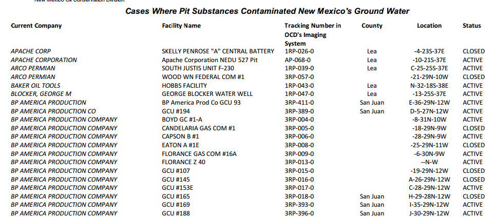
This 2008 document from the New Mexico Oil Conservation Division shows instances of ground water contamination by oil and gas pits in the state.
There isn’t much description on the document or the New Mexcio Oil Conservation Division (NMOCD) page that links to it, however, the subject matter is straightforward enough. Altogether, there are 369 instances of ground water contamination documented by a New Mexico governmental agency from dozens of drilling operators throughout the Land of Enchantment.
Ground Water Contamination Controversy
Since the title of document indicates that the agents causing contamination are “pit substances”, this does not technically indicate that hydraulic fracturing is to blame. This is largely a matter of definition, but it is an important one to understand, because the word “fracking” means something different to industry insiders than it does to the general public, and the issue of ground water contamination is a point of considerable debate.
Technically speaking, hydraulic fracturing only refers to one stage of the well completion process, in which water, sand, and chemicals are injected into the oil or gas well, and pressurized to break up the carbon-rich rock formation to allow the desired product to flow better.Most people (and many media outlets) consider “fracking” to be the entire production process for wells that require such treatment, from the development of the several acre well pad, through the drilling, the completion, flaring, waste disposal, and integration of the product to pipelines. (It is due to these competing definitions that the FracTracker Alliance goes out of our way to avoid the term “fracking”.)
All of this has lead to some carefully worded statements that seem to exhonerate hydraulic fracturing, despite suspected contamination events reported in Pennsylvania, Wyoming, and elsewhere. Of course, from the perspective of residents relying on a contaminated aquifer, it hardly matters whether the water was contaminated by hydraulic fracturing, leeching from the associated pits, problems with well casing or cement, or re-pressurized abandoned wells. A fouled aquifer is a fouled aquifer.
This document does not specify what was contained in the pits, only that they are contamination events. Therefore, we do not know what stage of the process the contaminant came from, only that it was believed by the state of New Mexico to have originated from a pit, and not the well bore itself.
Notes About Location Information
It is important to note that the location information is not exact, but are generally within 0.72 miles of the specified location. The reason for this is that the location information was provided using the Public Land Survey System (PLSS). The brainchild of Thomas Jefferson, the PLSS was the method used to grid out the western frontier, and it is still used as a legal land description in many western states. Essentially, the land was divided into townships that were six miles by six miles, which was then broken into 36 sections, each of which is one square mile. FracTracker has calculated the centroid of each section, which could be up to 0.71 miles from the corner of the same section if the shape is perfectly square.
The PLSS system was used to grid out most of New Mexico, but some portions of the state had already been well defined by Spanish and Mexcian land grants. Aside from being a fascinating historical anecdote, it does have an effect on the mapping of these pits. In the image of the table above, note that the “Florance Z 40” well does not have any values in the location column. As a result, we were not able to map this pit. Altogether, 11 of the 369 pits identified as causing groundwater contamination could not be mapped.
New Mexico Shale Viewer. You can zoom and click on map icons in this window for more information. For full access to map controls, including layer descriptions, please click the expanding arrows icon in the top right portion of the map.


")


. - Click to enlarge")
 - Click to enlarge")