Working with the environmental nonprofit Earthworks, FracTracker Alliance filmed emissions from oil and gas sites that have been issued permits in California under Governor Gavin Newsom since the beginning of 2019. Using state-of-the-art technology called optical gas imaging (OGI), we documented otherwise invisible toxic pollutants and greenhouse gas emissions (GHGs) being released from oil and gas wells and other infrastructure. This powerful technology provides further evidence of the negative consequences that come from each issued permit. Every single permit approval enabled by decisions made under Newsom can have substantial, visible impacts on local and regional air quality, contributes to climate change, and potentially exposes communities to health-harming pollution.
Despite a stated commitment to transition rapidly off fossil fuels, California has issued 7,625 permits to drill new oil and gas wells and rework existing wells since the beginning of 2019 — that is, on Governor Gavin Newsom’s watch. This expansion of the industry has clear implications for climate change and public health, as this article will demonstrate.
Intro
In collaboration with Consumer Watchdog, FracTracker Alliance has been periodically reporting on the number and locations of oil and gas wells permitted by Governor Newsom in California. In July of 2019, we showed how the rate of fracking under Governor Newsom had doubled, as compared to counts under former Governor Brown. Since then we have continued tracking the numbers and updating the California public via multiple news stories, blog reports, and with a map of new permits on NewsomWellWatch.com, where permitting data for the third quarter of 2020 has just been posted.
Now again, the rate of new oil and gas well permits issued by the California Geologic Energy Management division (CALGEM) continues to increase even faster in 2020, with permits issued to drill new oil and gas production wells nearly doubling since 2019. But what exactly does this mean for Frontline Communities and climate change? To answer this question, FracTracker Alliance and Consumer Watchdog teamed up with Earthworks’ Community Empowerment Project (CEP).
CEP’s California team worked with community members and grassroots groups to film emissions of methane and other volatile organic compounds (VOCs) emitted from oil and gas extraction sites, including infrastructure servicing oil and gas production wells such as the well-heads, separators, compressors, crude oil and produced water tanks, and gathering lines. Emissions of GHGs, such as methane, are a violation of the California Air Resources Board’s (CARB) California oil and gas rule (COGR), California Code of Regulations, Title 17, Division 3, Chapter 1, Subchapter 10 Climate Change, Article 4, § 95669, Leak Detection and Repair.
The emissions were filmed by a certified thermographer with a FLIR (Forward Looking Infrared) GF320 camera that uses optical gas imaging (OGI) technology. The OGI technology allows the camera to film and record visualizations of VOC emissions based on the absorption of infrared light. It is the exact same technology required by the U.S. EPA under the rule for new source performance standards and the by California Air Resources Board for Leak Detection and Repair (LDAR) to properly inspect oil and gas infrastructure. The video footage clearly shows the presence of a range of VOCs, methane, and other gases that are otherwise invisible to the naked eye.
The footage shown below is in greyscale and can appear grainy when the camera is being operated in high sensitivity modes, which is sometimes necessary to visualize certain pollution releases. The descriptions preceding each video explain what the trained camera operator saw and documented. A map of these sites is presented at NewsomWellWatch.com.
Newsom Well Watch interactive map
Navigate to the next slide using the arrows at the bottom of the map.
Find the story map, and more by clicking the image below.
Case Studies on Permitted Sites
Cat Canyon Tunnell Well Pad.
Earthworks’ California CEP thermographer visited this site in December of 2019, and just happened to arrive while the operator (oil and gas company) was conducting activities underground, including drilling new wells and reworking existing wells. In 2019 the operator, Vaquero Energy, was approved to drill 10 new cyclic steam wells and rework 23 existing oil and gas production wells at this site.
The footage shows significant emissions coming from an unknown source near the wellheads on the well pad; most likely these emissions were coming directly from the open boreholes of the wells. The emissions potentially include a cocktail of VOCs and GHGs such as methane, ethane, benzene, and toluene. This footage provides a candid view of what is released during these types of activities. The pollution shown appears to be the result of an uncontrolled source commonly resulting from drilling and reworking wells
Additionally, inspectors are rarely, if ever, present during these types of activities to ensure that they are conducted in accordance with regulations. The CEP camera operator reported the emissions and provided the OGI video to the Santa Barbara County Air Pollution Control District. By the time the inspector arrived, however, the drilling crew had ceased operations. The inspector did not detect any of these emissions, and as a result the operator was not held accountable for this large pollution release.
In the footage below, the emissions can be seen traveling over the fenceline of the well pad, swirling and mixing with the wind. This site is a clear example of what to look for in the following videos, since the emissions are so obvious. Fortunately, there are no homes or buildings in close proximity to this site, which potentially limited direct pollution exposure — although the pollution still degrades air quality and can pose an occupational health risk to oil field workers.
South Los Angeles Murphy Drill Site
The Murphy Drill Site in Los Angeles has been a long-standing nuisance and source of harmful pollution for neighbors in Jefferson Park. The site houses 31 individual operational wells, including 9 enhanced oil recovery injection wells and 22 oil and gas production wells, as shown below in the map in Figure 1. The wells are operated by Freeport-McMoran, while the site is owned by the Catholic archdiocese of Los Angeles. The site is within 200 feet of homes, playgrounds and a health clinic. There are over 16,000 residents within 2,500’ of the site, as well as a special needs high school, an elementary school, a hospice facility, and a senior housing complex.
Figure 1. Map of the Murphy drill site
The neighborhoods near the Murphy Site are plagued with strong chemical odors, including those linked to oil and gas operations (such as the “rotten egg” smell of health-harming hydrogen sulfide), most likely from the toxic waste incinerators on site. Community members have suffered from respiratory problems, chronic nosebleeds, skin and eye irritation, and headaches. The operators have received multiple violations, including for releasing emissions at concentrations 400% over the allowable limit of methane and VOCs. Some of these violations were the direct result of complaints from the community and the Earthworks CEP team, which filmed pollution from the site on multiple occasions. Yet despite receiving “Notices of Violations” and fines, Freeport-McMoran has been allowed to continue operations. In OGI footage, emissions are visible continuously escaping from a vent on the equipment. While this leak has been addressed by regulators, each new visit to this site tends to result in finding new uncontrolled emissions sources.
South Los Angeles Jefferson Drill Site
The Jefferson drill site is very similar situation to the Murphy Site. The sites have the same operator, Freeport-McMoran, and surrounding neighborhoods in both locations have suffered from exposure to toxic pollution as well as odors, truck traffic, and noise. The Jefferson site has 49 operational wells, including 15 enhanced oil recovery wells, as shown below in Figure 2. In 2013 the operator reported using over 130,000 pounds of corrosive acids and other toxic chemicals for enhanced oil recovery operations. Regardless, an environmental impact report has never been completed for this site.
Figure 2. Map of the Jefferson drill site in South Los Angeles.
The site is located 3 feet from the nearest home, and the surrounding residential buildings are considered “buffers” for the rest of the neighborhood, which also includes an elementary school about 700 feet away. The site was nearly shut down by the City of Los Angeles in 2019, but is currently still operational. In 2019 the site was even issued a permit to rework an existing well in order to increase production from the site. The footage below shows a large, consistent release of pollution from equipment on the well pad. The plume appears above the site and is visible against the background of the sky. The Earthworks CEP team reported the pollution to the South Coast Air Quality Management District (SCAQMD), which conducted an inspection, stopped the leak, and issued a notice of violation and a fine. It is not clear exactly how long this pollution problem had gone unnoticed or unaddressed, and it is not unlikely that another leak will occur without being quickly identified.
Wilmington E&B Resources WNF-I Site on Main St
The WNF-I drilling site is located in Carson in the City of Los Angeles. Operated by E&B Natural resources in the Wilmington oil and gas field, the site houses 35 operational oil and gas wells, including 12 enhanced oil recovery wells and a wastewater disposal well. There is also extensive above-ground infrastructure on the well site, including a large, high-volume tank battery used to store oil and wastewater produced from numerous oil and gas wells in the area.
Using OGI, Earthworks identified a large pollution release from the top of the largest tank. In the video footage, the plume or cloud of gases (likely methane and VOCs) can be seen hovering over the site and slowly dispersing over the fence-line into the communities of West Carson and Avalon Village. Despite clear operational problems, CalGEM approved this site for two rework permits in 2019 and then three re-drills (known as sidetracks) of existing wells in 2020 in order to increase production. The SCAQMD reports that they have inspected this facility, but it is not clear whether this major uncontrolled source has been stopped.
Long Beach Signal Hill Drill Site
At an urban drilling site in the neighborhood of Signal Hill in Los Angeles County, Earthworks filmed and documented pollution releases from numerous pieces of equipment. The site includes 15 operational oil and gas wells operated by Signal Hill Petroleum and The Termo Company. Emissions of gases (likely methane and VOCs) were documented on infrastructure from both operators. At this site, Signal Hill Petroleum received a permit in April 2019 to rework an operational well to increase production. That well is located less than 70’ from a home.
While this site is located within Los Angeles County, it is outside the jurisdiction of the city itself. Any local protections for drilling sites within the Los Angeles city limits are not afforded to communities such as Signal Hill. This area that includes the Signal Hill oil field and the Signal Hill portion of the Long Beach oil field, where many well sites are unmaintained and oversight is limited — conditions that in turn can result in corrosion and pollution leaks. The SCAQMD inspected this site and reported that these uncontrolled sources of emissions have been addressed by the operator, but it is not clear if the emission have stopped.
Midway-Sunset Crail Tank Farm
This tank farm, located in Kern County, services a number of wells operated by Holmes Western Oil Corporation on the outskirts of the Mid-Way Sunset Field. Of the wells serviced by this site, permits were issued to four active oil and gas production wells in 2019. The permits authorized the operator to rework the wellbores in order to increase production. The site contains nine operational oil and gas wells, including eight production wells pumping oil to the surface and one wastewater disposal well. There are multiple homes near this site, within 400’ to the west and within 300’ to the northeast.
For each gallon of oil produced, another ten gallons of contaminated wastewater are brought to the surface. Using diesel or gas generators this wastewater is pumped back into the ground. California regulators have a bad track record of managing underground injection of wastewater, which is now under the U.S. EPA’s oversight. The groundwater in this area of Kern County is largely contaminated and considered a sacrifice zone.
The emissions from this site are from the pressure release valves on the tops of multiple tanks. The tanks store both crude oil and wastewater. The infrared spectrum allows the camera to film the tank levels, which are nearly full. As the tanks fill with more crude oil and hydrocarbon contaminated wastewater the head space of the tank pressurizes with more VOC’s. This footage was also filmed at night when emissions are typically much lower. During the day heat from the sun (radiative energy) heats the tanks and increases the head space pressure resulting in greater emissions. While the San Joaquin Valley Air Pollution Control District (SJVAPCD) was notified of these uncontrolled sources of emissions, their own inspections of the site did not identify an actionable offense on the part of the operator and these uncontrolled emissions continue to be released.
Tank Emissions
Crude oil and wastewater storage tanks are a common source of fugitive emissions and represent the majority of emissions presented in this report. Some tanks and well-sites use best practices that include closed vapor recovery systems to prevent venting tanks from leaking, but the vast majority do not and vent directly to the atmosphere. In all cases, tanks and pipeline infrastructure use pressure release valves to vent emissions when pressure builds too high. This venting is permitted as strictly an emergency activity to prevent hazardous build-up of pressure. Vents are even designed to open and reset themselves automatically. Consequently, tank venting is a common practice and operators seem to often leave these valves open.
While the recently enacted California Oil and Gas Rule (COGR) places limits on GHG emissions from all oil and gas facilities, internal policy of the San Joaquin Air Valley Air Pollution Control District has previously exempted tanks at low-producing well sites from having to be kept in a leak-free condition, creating a regulatory conflict that air districts and CARB need to resolve. This type of emissions source is also difficult for regulators to identify during inspections, for a number of reasons. These valves are typically located on the tops of large tanks where they are difficult to access and view, and inspections and sampling can only occur by chance (i.e., when the valve in open). Further, these valves can be immediately closed by operators during or upon notification of an upcoming inspection.
New Permits: Moving in the Wrong Direction
When Earthworks CEP uses OGI cameras to inspect an oil and gas site in California, finding and documenting pollution releases is so common that it is the default expectation. Because of access and proximity limitations, it is possible that more pollution is being released from sites than CEP can identify. All of these examples of pollution, including releases of methane and VOCs, add up to potentially degrade air quality and expose Frontline Communities to health risks — as well as many others just like them. This summary represents a small collection of leaking well sites visited by Earthworks CEP, which have coincidentally received new permits to operate and rework existing wells since January 1, 2019. CEP has also documented many other hazardous cases, such as the Jewett 1-23 site in Arvin (shown in the footage below), that is persistently exposing elementary school students to VOCs. These sites surely make up only a small proportion of the polluting oil and gas sites in California that harm climate and health.
From the initial drilling of an oil and gas well, during production, and into subsequent reworks, all phases of a well’s lifetime result in unpermitted and undocumented fugitive emissions. Regulating emissions from oil and gas extraction operations has not been effective in California. Regardless of notices of violations and fines, polluting facilities and well sites continue to operate and even receive new permits. Even the COGR rule, lauded as the most stringent GHG emissions regulation in the nation is technically unable to eliminate or even identify these uncontrolled sources. It is clear that the only ways to reduce exposures to these emissions for Frontline Communities is to institute protective setbacks and stop permitting the drilling of new wells and the reworking of aging wells.
https://www.fractracker.org/a5ej20sjfwe/wp-content/uploads/2019/08/EQT-Tioga-Wide-7.gif300800Kyle Ferrar, MPHhttps://www.fractracker.org/a5ej20sjfwe/wp-content/uploads/2025/09/2025-Wordmark-Logo.pngKyle Ferrar, MPH2020-11-18 12:40:132021-04-15 14:16:04Documenting emissions from new oil and gas wells in California
In this article, we’ll take a look at the current trend in “re-branding” incineration as a viable option to deal with the mountains of garbage generated by our society. Incineration can produce energy for electricity, but can the costs—both economically, and ecologically—justify the benefits? What are the alternatives?
Changes in our waste stream
In today’s world of consumerism and production, waste disposal is a chronic problem facing most communities worldwide. Lack of attention to recycling and composting, as well as ubiquitous dependence on plastics, synthetics, and poorly-constructed or single-use goods has created a waste crisis in the United States. So much of the waste that we create could be recycled or composted, however, taking extraordinary levels of pressure off our landfills. According to estimates in 2017 by the US Environmental Protection Agency (EPA), over 30 percent of municipal solid waste is made up of organic matter like food waste, wood, and yard trimmings, almost all of which could be composted. Paper, glass, and metals – also recyclable – make up nearly 40 percent of the residential waste stream. Recycling plastic, a material which comprises 13% of the waste stream, has largely been a failed endeavor thus far.
Why say NO to incinerators?
They are bad for the environment, producing toxic chlorinated byproducts like dioxins. Incineration often converts toxic municipal waste into other forms, some of which are even more toxic than their precursors.
They often consume more energy than they produce and are not profitable to run.
They add CO2 to the atmosphere.
They promote the false narrative that we can “get something” from our trash
They detract from the conversation about actual renewable energy sources like wind power, solar power, and geothermal energy that will stop the acceleration of climate chaos.
Nevertheless, of the approximately 400 million tons of plastic produced annually around the world, only about 10% of it is recycled. The rest winds up in the waste stream or as microfragments (or microplastics) in our oceans, freshwater lakes, and streams.
According to an EPA fact sheet, by 2017, municipal solid waste generation increased three-fold compared with 1960. In 1960, that number was 88.1 million tons. By 2017, this number had risen to nearly 267.8 million tons. Over that same period, per-capita waste generation rose from 2.68 pounds per person per day, to 4.38 pounds per person per day, as our culture became more wed to disposable items.
The EPA provides a robust “facts and figures” breakdown of waste generation and disposal here. In 2017, 42.53 million tons of US waste was shipped to landfills, which are under increasing pressure to expand and receive larger and larger loads from surrounding area, and, in some cases, hundreds of miles away.
How are Americans doing in reducing waste?
On average, in 2017, Americans recycled and composted 35.2% of our individual waste generation rate of 4.51 pounds per person per day. While this is a notable jump from decades earlier, much of the gain appears to be in the development of municipal yard waste composting programs. Although the benefits of recycling are abundantly clear, in today’s culture, according to a PEW Research Center report published in 2016, just under 30% of Americans live in communities where recycling is strongly encouraged. An EPA estimate for 2014 noted that the recycling rate that year was only 34.6%, nationwide, with the highest compliance rate at 89.5% for corrugated boxes.
Figure 3. Percent of Americans who report recycling and re-use behaviors in their communities, via Pew Research center
Historically, incineration – or burning solid waste – has been one method for disposing of waste. And in 2017, this was the fate of 34 million tons—or nearly 13%– of all municipal waste generated in the United States. Nearly a quarter of this waste consisted of containers and packaging—much of that made from plastic. The quantity of packaging materials in the combusted waste stream has jumped from only 150,000 tons in 1970 to 7.86 million tons in 2017. Plastic, in its many forms, made up 16.4% of all incinerated materials, according to the EPA’s estimates in 2017.
Figure 4: A breakdown of the 34.03 tons of municipal waste incinerated for energy in the US in 2017
What is driving the abundance of throw-away plastics in our waste stream?
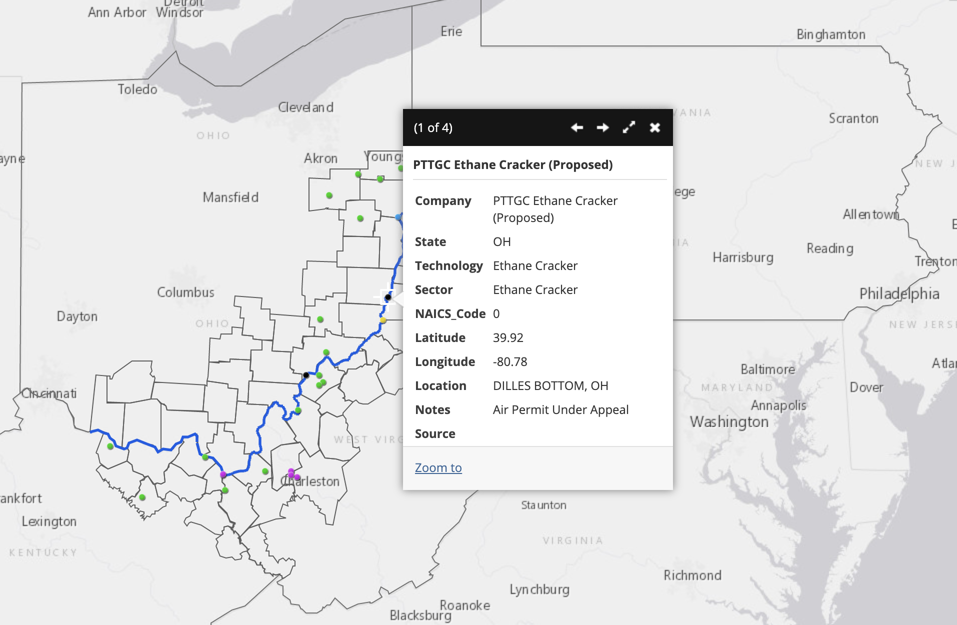
Sadly, the answer is this: The oil and gas industry produces copious amounts of ethane, which is a byproduct of oil and gas extraction. Plastics are an “added value” component of the cycle of fossil fuel extraction. FracTracker has reported extensively on the controversial development of ethane “cracker” plants, which chemically change this extraction waste product into feedstock for the production of polypropylene plastic nuggets. These nuggets, or “nurdles,” are the building blocks for everything from fleece sportswear, to lumber, to packaging materials. The harmful impacts from plastics manufacturing on air and water quality, as well as on human and environmental health, are nothing short of stunning.
FracTracker has reported extensively on this issue. For further background reading, explore:
A report co-authored by FracTracker Alliance and the Center for Environmental Integrity in 2019 found that plastic production and incineration in 2019 contributed greenhouse gas emissions equivalent to that of 189 new 500-megawatt coal power plants. If plastic production and use grow as currently planned, by 2050, these emissions could rise to the equivalent to the emissions released by more than 615 coal-fired power plants.
Just another way of putting fossil fuels into our atmosphere
Incineration is now strongly critiqued as a dangerous solution to waste disposal as more synthetic and heavily processed materials derived from fossils fuels have entered the waste stream. Filters and other scrubbers that are designed to remove toxins and particulates from incineration smoke are anything but fail-safe. Furthermore, the fly-ash and bottom ash that are produced by incineration only concentrate hazardous compounds even further, posing additional conundrums for disposal.
Incineration as a means of waste disposal, in some states is considered a “renewable energy” source when electricity is generated as a by-product. Opponents of incineration and the so-called “waste-to-energy” process see it as a dangerous route for toxins to get into our lungs, and into the food stream. In fact, Energy Justice Network sees incineration as:
… the most expensive and polluting way to make energy or to manage waste. It produces the fewest jobs compared to reuse, recycling and composting the same materials. It is the dirtiest way to manage waste – far more polluting than landfills. It is also the dirtiest way to produce energy – far more polluting than coal burning.
Municipal waste incineration: bad environmentally, economically, ethically
Waste incineration has been one solution for disposing of trash for millennia. And now, aided by technology, and fueled by a crisis to dispose of ever-increasing trash our society generates, waste-to-energy (WTE) incineration facilities are a component in how we produce electricity.
But what is a common characteristic of the communities in which WTEs are sited? According to a 2019 report by the Tishman Environmental and Design Center at the New School, 79% of all municipal solid waste incinerators are located in communities of color and low-income communities. Incinerators are not only highly problematic environmentally and economically. They present direct and dire environmental justice threats.
Waste-to-Energy facilities in the US, existing and proposed
Activate the Layers List button to turn on Environmental Justice data on air pollutants and cancer occurrences across the United States. We have also included real-time air monitoring data in the interactive map because one of the health impacts of incineration includes respiratory illnesses. These air monitoring stations measure ambient particulate matter (PM 2.5) in the atmosphere, which can be a helpful metric.
What are the true costs of incineration?
These trash incinerators capture energy released from the process of burning materials, and turn it into electricity. But what are the costs? Proponents of incineration say it is a sensible way to reclaim or recovery energy that would otherwise be lost to landfill disposal. The US EIA also points out that burning waste reduces the volume of waste products by up to 87%.
The down-side of incineration of municipal waste, however, is proportionally much greater, with a panoply of health effects documented by the National Institutes for Health, and others.
Dioxins (shown in Figures 6-11) are some of the most dangerous byproducts of trash incineration. They make up a group of highly persistent organic pollutants that take a long time to degrade in the environment and are prone to bioaccumulation up the food chain.
Dioxins are known to cause cancer, disrupt the endocrine and immune systems, and lead to reproductive and developmental problems. Dioxins are some of the most dangerous compounds produced from incineration. Compared with the air pollution from coal-burning power plants, dioxin concentrations produced from incineration may be up to 28 times as high.
Federal EPA regulations between 2000 and 2005 resulted in the closure of nearly 200 high dioxin emitting plants. Currently, there are fewer than 100 waste-to-energy incinerators operating in the United States, all of which are required to operate with high-tech equipment that reduces dioxins to 1% of what used to be emitted. Nevertheless, even with these add-ons, incinerators still produce 28 times the amount of dioxin per BTU when compared with power plants that burn coal.
Even with pollution controls required of trash incinerators since 2005, compared with coal-burning energy generation, incineration still releases 6.4 times as much of the notoriously toxic pollutant mercury to produce the equivalent amount of energy.
Energy Justice Network, furthermore, notes that incineration is the most expensive means of managing waste… as well as making energy. This price tag includes high costs to build incinerators, as well as staff and maintain them — exceeding operation and maintenance costs of coal by a factor of 11, and nuclear by a factor of 4.2.
Figure 12. Costs of incineration per ton are nearly twice that of landfilling. Source: National Solid Waste Management Association 2005 Tip Fee Survey, p. 3.
Energy Justice Network and others have pointed out that the amount of energy recovered and/or saved from recycling or composting is up to five times that which would be provided through incineration.
Figure 13. Estimated power plant capital and operating costs. Source: Energy Justice Network
The myth that incineration is a form of “renewable energy”
Waste is a “renewable” resource only to the extent that humans will continue to generate waste. In general, the definition of “renewable” refers to non-fossil fuel based energy, such as wind, solar, geothermal, wind, hydropower, and biomass. Synthetic materials like plastics, derived from oil and gas, however, are not. Although not created from fossil fuels, biologically-derived products are not technically “renewable” either.
Biogenic materials you find in the residual waste stream, such as food, paper, card and natural textiles, are derived from intensive agriculture – monoculture forests, cotton fields and other “green deserts”. The ecosystems from which these materials are derived could not survive in the absence of human intervention, and of energy inputs from fossil sources. It is, therefore, more than debatable whether such materials should be referred to as renewable.
Although incineration may reduce waste volumes by up to 90%, the resulting waste-products are problematic. “Fly-ash,” which is composed of the light-weight byproducts, may be reused in concrete and wallboard. “Bottom ash” however, the more coarse fraction of incineration—about 10% overall—concentrates toxins like heavy metals. Bottom-ash is disposed of in landfills or sometimes incorporated into structural fill and aggregate road-base material.
How common is the practice of using trash to fuel power plants?
Trash incineration accounts for a fraction of the power produced in the United States. According to the United States Energy Information Administration, just under 13% of electricity generated in the US comes from burning of municipal solid waste, in fewer than 65 waste-to-energy plants nation-wide. Nevertheless, operational waste-to-incineration plants are found throughout the United States, with a concentration east of the Mississippi.
According to EnergyJustice.net’s count of waste incinerators in the US and Canada, currently, there are:
88 operating
41 proposed
0 expanding
207 closed or defeated
Figure 14. Locations of waste incinerators that are already shut down. Source: EnergyJustice.net)
Precise numbers of these incinerators are difficult to ascertain, however. Recent estimates from the federal government put the number of current waste-to-energy facilities at slightly fewer: EPA currently says there are 75 of these incinerators in the United States. And in their database, updated July 2020, the United States Energy Information Administration (EIA), lists 63 power plants that are fueled by municipal solid waste. Of these 63 plants, 40—or 66%—are in the northeast United States.
Regardless, advocates of clean energy, waste reduction, and sustainability argue that trash incinerators, despite improvements in pollution reduction over earlier times and the potential for at least some electric generation, are the least effective option for waste disposal that exists. The trend towards plant closure across the United States would support that assertion.
Let’s take a look at the dirty details on WTE facilities in three states in the Northeastern US.
Review of WTE plants in New York, Pennsylvania, and New Jersey
A. New York State
Operational WTE Facilities
In NYS, there are currently 11 waste-to-energy facilities that are operational, and two that are proposed. Here’s a look at some of them:
The largest waste-to-energy facility in New York State, Covanta Hempstead Company (Nassau County), was built in 1989. It is a 72 MW generating plant, and considered by Covanta to be the “cornerstone of the town’s integrated waste service plan.”
According to the Environmental Protection Agency’s ECHO database, this plant has no violations listed. Oddly enough, even after drawing public attention in 2009 about the risks associated with particulate fall-out from the plant, the facility has not been inspected in the past 5 years.
Other WTE facilities in New York State include the Wheelabrator plant located in Peekskill (51 MW), Covanta Energy of Niagara in Niagara Falls (32 MW), Convanta Onondaga in Jamesville (39 MW), Huntington Resource Recovery in Suffolk County (24.3 MW), and the Babylon Resource Recovery Facility also in Suffolk County (16.8 MW). Five additional plants scattered throughout the state in Oswego, Dutchess, Suffolk, Tioga, and Washington Counties, are smaller than 15 MW each. Of those, two closed and one proposal was defeated.
Closed / Defeated Facilities
The $550 million Corinth American Ref-Fuel, was proposed for Corinth, New York. It was designed to take 1.27 million tons of New York City waste/year, even more than what is planned for the CircularEnerG plant. It was defeated ~2004. Population of 864 in immediate vicinity of plant, 98% white, income $59K.
Fire Island, Saltaire Incinerator closed. Took 12 tons/day. It was opened in 1965s, but not designed to produce energy, just burn trash. There was a population of 317 in immediate vicinity of plant, 93% white, income $123K.
The Long Beach incinerator processed 200 tons per day of solid waste. This plant was operating in 1988, but closed in 1996.
The Albany Steam Plant closed in 1994. When it was operational, it took in 340-600 tons of trash per day. Environmental justice issues were plentiful at this plant, with over 99% of the area as African American, according to the LA Times coverage of the issue.
CircularEnerG, was a 50 MW plant proposed in Romulus, on the former Seneca Army Depot, in the middle of largely white Seneca County, New York. However, the nearest large population to the proposed site was the 1500-prisoner capacity Five Points Correctional facility, swaying the demographics to nearly 52% African American in the highest impact zone. More broadly, the facility was in the heart of the Finger Lakes wine region, known for its extraordinary scenery, clean lakes, and award-winning wines. This facility was broadly opposed by nearly all the surrounding municipalities and counties, and mired in controversy about improper procedures and a designation by a local zoning officer as a “renewable” source of energy in its early filing papers.
Local advocacy groups, Seneca Lake Guardian (an affiliate of the Waterkeeper Network), and the Finger Lakes Wine Business Coalition worked exhaustively with the legal group, Earthjustice, to stop the project.
Figure 15. Map of regional governments and organizations opposed to construction of Romulus waste-to-energy incinerator in New York State
In March 2019, after state lawmakers, along with Governor Andrew Cuomo came out against the trash incinerator, the special use permit application for the facility was withdrawn.
Plans were also in development for a garbage-to-gas plant in the Hudson River community of Stony Point, New York. The company, New Planet Energy, had hoped to construct the gasification plant that would accept 4,500 tons of waste daily, brought in each day by approximately 400 trucks, according to an article in Lohud, May 1, 2018. However, the owner of the property eventually backed out of the proposal shortly after the publication of the article, following an uptick in criticism about the project about environmental and traffic safety concerns. This property is also currently an active Superfund site.
Proposed WTE Facilities
In New York State, there are currently two proposed WTE facilities.
New York State has rejected the designation for WTE facilities since 2011. As of the latest reports, the company is pushing ahead with its plans, despite the widespread dislike for the project. A bill in the State Legislature has been introduced to block the project. Green Waste Energy has been proposed for Rensselaer, NY. This trash-burning gasification plant would accept 2500 tons of trash per day. However, in August 2020, the New York State Department of Environmental Conservation (DEC) denied the air quality permit for the facility. The developers may appeal this decision.
In New Windsor, NY, a project called W2E Orange County has been under consideration. Most recent news coverage of this project was three and a half years ago, so it is possible this project is not moving forward. The parent company of the project, Ensorga, appears to have contracted its operations to West Virginia.
B. Pennsylvania
Operational WTE Facilities
In Pennsylvania, six WTE facilities are currently operating. Two have been closed, and six defeated.
Proposed WTE Facilities
In Pennsylvania, there are currently no WTEs under consideration for construction.
Closed WTE Facilities
Chester Resource Recovery #1 was used from the late 1950s to 1979. The neighborhood is over 64% African American. This was one of three incinerators used here.
Westmoreland County WTE plant, which opened in 1986 and burned 25 tons of solid municipal waste per day, has been closed due to financial unviability, and lack of need for the steam that was produced, according to a report drafted in 1997. It was located in a densely populated area, and provided steam to a nursing home, jail, and low-income housing.
Defeated WTE Facility Proposals
Elroy trash-to-steam plant was located in a densely populated section of Franconia Township, Montgomery County, Pennsylvania. It was to handle 360 tons of waste per day and was located on the grounds of a rendering plant. The application for this plant was withdrawn in June, 1989. Citizens for a Clean Environment successfully defeated this project.
The Plasma Gasification Incinerator, located in Hazle Township, Pennsylvania, was proposed to burn 4,000 tons of trash per day. The median income in the immediate vicinity of the site is $46K. The application for this project was withdrawn.
The Pittston Trash Incinerator in a very low-income area of Luzerne County, Pennsylvania, was designed to burn 3,000 tons of trash per day. This project was defeated.
The $65 million Delta Thermo Muncy facility, which would have burned municipal waste and sewage sludge, was defeated in December, 2016. Citizens in the Energy Justice Network and Stop the Muncy Waste Incinerator organized and passed a set-back ordinance that made it impossible for the plant to locate there. This proposed plant, would have been located in Lycoming County, Pennsylvania. The plan there was to decompose trash and sewage through a hydrothermal technique to create pellets, which would then be burned to yield energy.
Originally proposed in 2007, the $49 million Delta Thermo Allentown plant has been fought for many years by Allentown Residents for Clean Air. If built, it would generate 2 MW of energy, and receive 100 tons of municipal waste each day and 50 tons of sewage sludge. The plant is located in a densely-populated, predominately Hispanic neighborhood. There has been no news on this project in over four years, so this project appears to have been defeated.
Glendon Energy proposed building an incinerator in Northampton County, Pennsylvania. This proposal was also defeated.
C. New Jersey
Operational WTE Facilities
And in New Jersey, there are currently four operating WTE facilities. Essex County Resource Recovery Facility, is New Jersey’s largest WTE facility. It opened in 1990, houses three burners, and produces 93 MW total.
Three WTE facilities are currently proposed in New Jersey. Jefferson Renewable Energy Trash Incinerator (Jersey City, New Jersey) is designed to produce 90 MW of power, accepting 3,200 tons/day solid waste, plus 800 tons/day construction/demo waste.
Delta Thermo Sussex is designed to burn both municipal solid waste and sewage sludge. And DTE Paterson would accept 205 tons of waste/day. The price tag to build this small facility is not so small: $45 million.
Closed WTE Facilities
Two WTE plants in New Jersey are no longer in operation. These include Fort Dix, which opened in 1986 and burned 80 tons of trash per day; and Atlantic County Jail, which opened in 1990 and burned 14 tons of trash per day.
Throw-aways, burn-aways, take-aways
Looming large above the arguments about appropriate siting, environmental justice, financial gain, and energy prices, is a bigger question:
How can we continue to live on this planet at our current rates of consumption, and the resultant waste generation?
The issue here is not so much about the sources of our heat and electricity in the future, but rather “How MUST we change our habits now to ensure a future on a livable planet?”
Professor Paul Connett (emeritus, St. Lawrence University), is a specialist in the build-up of dioxins in food chains, and the problems, dangers, and alternatives to incineration. He is a vocal advocate for a “Zero Waste” approach to consumption, and suggests that every community embrace these principles as ways to guide a reduction of our waste footprint on the planet. The fewer resources that are used, the less waste is produced, mitigating the extensive costs brought on by our consumptive lifestyles. Waste-to-energy incineration facilities are just a symptom of our excessively consumptive society.
Dr. Connett suggests these simple but powerful methods to drastically reduce the amount of materials that we dispose — whether by incineration, landfill, or out the car window on a back-road, anywhere in the world:
Source separation
Recycling
Door-to-door collection
Composting
Building Reuse, Repair and Community centers
Implementing waste reduction Initiatives
Building Residual Separation and Research centers
Better industrial design
Economic incentives
Interim landfill for non-recyclables and biological stabilization of other organic materials
Connett’s Zero Waste charge to industry is this: “If we can’t reuse, recycle, or compost it, industry shouldn’t be making it.” Reducing our waste reduces our energy footprint on the planet.
In a similar vein, FracTracker has written about the potential for managing waste through a circular economics model, which has been successfully implemented by the city of Freiburg, Germany. A circular economic model incorporates recycling, reuse, and repair to loop “waste” back into the system. A circular model focuses on designing products that last and can be repaired or re-introduced back into a natural ecosystem.
This is an important vision to embrace. Every day. Everywhere.
For more in-depth and informative background on plastic in the environment, please watch “The Story of Plastic” (https://www.storyofplastic.org/). The producers of the film encourage holding group discussions after the film so that audiences can actively think through action plans to reduce plastic use.
https://www.fractracker.org/a5ej20sjfwe/wp-content/uploads/2020/10/Waste-to-Energy-facilities-in-the-US-feature--scaled.jpg6671500Karen Edelsteinhttps://www.fractracker.org/a5ej20sjfwe/wp-content/uploads/2025/09/2025-Wordmark-Logo.pngKaren Edelstein2020-10-19 15:11:492021-04-15 14:16:05Incinerators: Dinosaurs in the world of energy generation
With this recent development, it is necessary to provide science-based recommendations for the EIR to prioritize the protection of the health of frontline communities. Frontline communities bear the most risk. Emissions from oil and gas infrastructure and exposure to water and soil contamination most affect those living closest. It is therefore vital for an EIR to institute protections that address these known and well-established sources of exposure. In addition, the EIR must prioritize a requirement by law that all regulatory information is equitably available and imparted to Frontline Communities; with Kern County, this means providing regulatory notices in Spanish, the predominantly spoken language in this area, according to household census data.
In preparation of the Kern County rule-making process, FracTracker Alliance has prepared new analyses of Kern County communities. These analyses have mapped and assessed the distribution of oil and gas wells within Kern County for proximity to sensitive receptors. This information is vital to understand how the “most drilled County” in the United States manages the risks associated with oil and gas extraction. According to CalGEM data updated September 1, 2020, there are 78,016 operational oil and gas wells countywide. Of these, 5,906 (7.6%) are within 2,500 feet of a sensitive receptor, receptors being homes, schools, healthcare facilities, child daycare facilities, and elderly care facilities. Thirty-six CHHS healthcare facilities and 35 schools in Kern County are within 2,500 feet of an operational oil and gas well. In fact, 646 operational wells are within 2,500 feet of a school in Kern County. Most of these at-risk, sensitive receptors are in Kern’s cities, large and small.
Table 1. Well Counts in Kern County
Most of the population of Kern County is in its cities. Unincorporated, rural areas of Kern County are in majority zoned for large estate landownership and agriculture, and have low population density, rather than designated for residential, single-family homes, apartments, developments, and mobile homes. Oil and gas extraction operations and well sites are dispersed throughout the county, including near and within the residentially-zoned areas of cities. Given that the county’s population density is highest in cities, these areas present the greatest public health risk for exposures to toxic emissions and spills from fossil fuel extraction operations. This analysis focuses specifically on the Frontline Communities of Kern County, where oil and gas extraction is occurring near city limits.
Table 2. Operational oil and gas well counts near cities and sensitive receptors.
Frontline Communities
These include Lost Hills, Lamont, Taft, Arvin, Shafter and Bakersfield. In Table 2 (above) are counts of operational wells within two miles of each city, along with demographic profiles for each incorporated/unincorporated city, based on American Community Survey (2013-2018) census data (downloaded from Census.gov). Population estimates are based on the ACS block groups. For block groups larger than city boundaries, the population was assumed to be within city limits, although in certain cases, such as Arvin, a small section of a block group was eliminated from the city demographic counts. This assumption is validated by the county and city zoning parcels. The maps below in Figures 1 – 6 show the municipal zoning parcels for these cities, with maps that include operational oil and gas wells. Note the proximity of residential- and urban-zoned parcels to oil and gas extraction in Kern County, and the difference in zoning between the cities and the rest of the county. Cities are zoned for residences, including apartments, single-family homes, and mobile homes. Most of the rest of the county is agriculture and estates, where predominantly wealthy residents and corporations own large holdings.
Figure 1. Municipal zoning boundaries of the City of Lost Hills.
Figure 2. Municipal zoning boundaries of the City of Lamont.
Figure 3. Municipal zoning boundaries of the City of Taft.
Figure 4. Municipal zoning boundaries of the City of Arvin.
Figure 5. Municipal zoning boundaries of the City of Shafter.
Figure 6. Municipal zoning boundaries of the City of Bakersfield.
Economic Disparity in Environmental Justice Communities
These six cities and their Frontline Communities experience a disparity of exposure to environmental pollutants, particularly emissions from oil and gas extraction operations — as well as pesticides, regionally degraded air quality (from ozone and particulate matter), and contaminated groundwater. Besides the risk disparity, these communities are also vulnerable from several other factors, including disparities in economic opportunity, demographics, and access to information.
Compared to the rest of Kern County, Frontline Communities in these unincorporated and incorporated cities have less financial opportunity. The maps in Figures 7 – 9 below show block groups and the proportions of the population with annual median incomes less than or equal to $40,000. This value was chosen because it is less than 80% of the countywide median income of $51,579 in 2018. For comparison, the statewide median income is $75,277. Lack of economic opportunity for these communities limits the ability to leverage financial resources to protect their community health and to maintain local-level financial independence from corporate influence. In Lost Hills, over 80% of the city block group closest to the Lost Hills Oil Field has a median income less than or equal to $40,000. The same trend is visible for Lamont, Taft, and Arvin. In Figure 9, the only section of Taft with higher annual median income is sparsely populated and predominantly open space, as confirmed in Figure 3. For the areas of Frontline Community block groups within 2,500 feet of an operational well, 36% of the population makes under $40,000; 80% of the Kern County annual median income is $41,000.
In the maps below, the American Community Survey data is summarized in percentages of one, where, for example, light orange (<.400) in the map refers to areas where 20% – 40% of the population’s annual median income is less than or equal to $40,000.
Table 3. Demographical Profile of each city, including the percentage of Spanish-speaking households and proportion of households with limited English proficiency.
Figure 7. Lost Hills income disparity: This map shows the population percentage with annual incomes of less than or equal to $40,000, which is less than 80% of the Kern median income of $51,579 (2018).
Figure 8. Lamont income disparity: This map shows the population percentage with annual incomes less than or equal to $40,000, which is less than 80% of the Kern median income of $51,579 (2018).
Figure 9. Taft income disparity: This map shows the population percentage with annual incomes less than or equal to $40,000, which is less than 80% of the Kern median income of $51,579 (2018).
Figure 10. Arvin income disparity: This map shows the population percentage with annual incomes less than or equal to $40,000, which is less than 80% of the Kern median income of $51,579 (2018).
Linguistic Isolation Disenfranchises Frontline Communities
Access to information is vital for representation. Without representation, communities have no power over their autonomy. Kern County’s Frontline Communities are denied this basic, but absolutely vital right. According to the U.S. Census, over 51% of Kern County is Hispanic, and the maps below show that the demographics of the Frontline Communities in these cities are regularly between 80 – 100% Hispanic. Additionally, the maps illustrate that the households in these communities are majority Spanish-speaking households, many with limited English proficiency (all persons aged five and older reported speaking English less than “very well”). Yet Kern County regulators only provide information, notices, and other materials in English. This linguistically segregates power in Kern County, limiting Spanish-speaking Kern residents and citizens from participating in local decision-making processes.
Using the five-year ACS census data (2018) clipped by the 2,500 feet well setback zone, I have calculated the percentage and number of Spanish-speaking households. For the areas of Frontline Community block groups within 2,500 feet of an operational well, 9,077 households (30.8%) speak Spanish as their primary language, and 1,900 households have limited access to proficient English translators.
Figure 11. Lost Hills Hispanic population demographics: This map shows the Hispanic percentage of the population. In these maps, the ACS data is summarized in percentages of one, where, for example, light orange (<.400) refers to areas where 20% – 40% of the population is Hispanic.
Figure 12. Lost Hills Spanish-speaking households: This map shows the percentage of the households that speak Spanish as their primary language. In these maps, the ACS data is summarized in percentages of one, where, for example, light orange (<.400) refers to areas where 20% – 40% of the households are Spanish speaking.
Figure 13. Lost Hills Limited English Spanish-speaking households: This map shows the household percentage that speak Spanish as their primary language, with limited English-speaking proficiency. In these maps, the ACS data is summarized in percentages of one, where, for example, light orange (<.400) refers to areas where 20% – 40% of the households are Spanish speaking and have limited English proficiency.
Figure 14. Lamont Hispanic population demographics: This map shows the Hispanic percentage of the population. In these maps, the ACS data is summarized in percentages of one, where, for example, light orange (<.400) refers to areas where 20% – 40% of the populations is Hispanic.
Figure 15. Lamont Spanish-speaking households: This map shows the percentage of the households that speak Spanish as their primary language. In these maps the ACS data is summarized in percentages of one, where, for example, light orange (<.400) refers to areas where 20% – 40% of the households are Spanish speaking.
Figure 16. Lamont Limited English Spanish-speaking households: This map shows the percentage of the households that speak Spanish as their primary language, with limited English-speaking proficiency. In these maps, the ACS data is summarized in percentages of one, where, for example, light orange (<.400) refers to areas where 20% – 40% of the households are Spanish speaking and have limited English proficiency.
Figure 17. Taft Hispanic population demographics: The map shows the Hispanic percentage of the population. In these maps the American Community Survey data is summarized in percentages of 1, where, for example, light orange (<.400) in the map below refers to areas where 20%-40% of the populations is Hispanic.
Figure 18. Taft Spanish-speaking households: This map shows the percentage of the households that speak Spanish as their primary language. In these maps, the ACS data is summarized in percentages of one, where, for example, light orange (<.400) refers to areas where 20% – 40% of the households are Spanish speaking.
Figure 19. Arvin Hispanic population demographics: This map shows the Hispanic percentage of the population. In these maps, the ACS data is summarized in percentages of one, where, for example, light orange (<.400) refers to areas where 20% – 40% of the populations is Hispanic.
Figure 20. Arvin Spanish-speaking households: This map shows the percentage of the households that speak Spanish as their primary language. In these maps, the ACS data is summarized in percentages of one, where, for example, light orange (<.400) refers to areas where 20% – 40% of the households are Spanish speaking.
Figure 21. Arvin Limited English Spanish-speaking households: This map shows the percentage of the households that speak Spanish as their primary language, with limited English-speaking proficiency. In these maps, the ACS data is summarized in percentages of one, where, for example, light orange (<.400) refers to areas where 20% – 40% of the households are Spanish speaking, with limited English proficiency.
Figure 22. Shafter Hispanic population demographics: This map shows the Hispanic percentage of the population. In these maps, the ACS data is summarized in percentages of one, where, for example, light orange (<.400) refers to areas where 20% – 40% of the populations is Hispanic.
Figure 23. Shafter Spanish-speaking households: This map shows the percentage of the households that speak Spanish as their primary language. In these maps, the ACS data is summarized in percentages of one, where, for example, light orange (<.400) refers to areas where 20% – 40% of the households are Spanish speaking.
Figure 24. Bakersfield Hispanic population demographics: This map shows the Hispanic percentage of the population. In these maps, the ACS data is summarized in percentages of one, where, for example, light orange (<.400) refers to areas where 20% – 40% of the populations is Hispanic.
Figure 25. Bakersfield Spanish-speaking households: This map shows the percentage of the households that speak Spanish as their primary language. In these maps, the ACS data is summarized in percentages of one, where, for example, light orange (<.400) refers to areas where 20% – 40% of the households are Spanish speaking.
Conclusions
These maps make it visually clear that the Frontline Communities near oil and gas extraction in Kern County are largely disenfranchised from the democratic process, a direct result of California’s regulatory agencies refusing to provide notices and other important documents and information in Spanish. Additionally, these same communities have limited options, due to economic disparities that make Kern County’s Frontline Communities the poorest in the state of CA. These two factors leveraged against communities prevent them from obtaining self-governance or autonomy over the industrialization occurring in and around their neighborhoods. Furthermore, the demarcations of census boundaries splitting the incorporated and unincorporated cities are essentially gerrymandered to disguise the blatant environmental inequities that exist in Kern County, in direct violation of the California Environmental Quality Act. Kern County must consider these injustices in the development of new environmental impact review requirements for oil and gas operators.
The following addendum incorporates additional demographics data that more thoroughly describes Frontline Communities in Kern County. We focus on the Frontline Communities closest to intense oil extraction operations. This analysis prioritizes areas with substantial population density. Remote sensing (satellite imagery) data and direct knowledge of Kern County cities was used to define the sample areas for this analysis. These techniques and methods avoid the type of spatial bias that distorted the results of the environmental justice (EJ) analysis inthe 2020 Kern County draft EIR (chapter 7 PDF pp.1292-1305).
2020 Kern County Draft EIR
The EJ analysis included in the 2020 Kern County Draft EIR uses the spatial bias of US census designated areas to generate false conclusions. The Draft EIR can do this in two ways:
First, the Draft EIR uses census tracts in the place of smaller census designated areas. The draft EIR states the county conducted, “an analysis of Kern County census tract five-year American Community Survey (ACS) demographic and poverty data for the period was conducted … and the five-year data is the most accurate form of ACS data, has the largest sample size, and is the only ACS data that covers tiny populations.” While this is true about the five-year data, the authors chose to analyze using census tracts, which are much too large to cover small populations. It is not clear why the authors would have chosen census tracts, rather than the higher resolution ‘census block groups’ ACS dataset, as both datasets are readily available from the US Census Bureau.
Additionally, the draft EIR limits the sociodemographic analysis to only census tracts that contain PLSS QTR/QTRS’s ranked as Tier 1, so that it does not include neighboring communities in different census tracts in the demographical analysis. As discussed in the draft EIR, Tier 1 areas contain four or more operational wells in a tiny area. The draft EIR explicitly states that Tier 1 Qtr(s) do not contain schools or healthcare facilities. This trend is not limited to just the Qtr/Qtr sections. The census tracts containing the Tier 1 sections contain very few sensitive receptors, like schools and healthcare facilities. This is because census tracts and other census designated areas are drawn specifically to differentiate between urban and rural/industrial areas. Census tracts containing oil fields cover large rural areas, and intentionally avoid areas with any significant population density. This results in donuts and other strange shapes, where communities in much smaller census tracts (by area) are enveloped by large rural census tracts containing oil fields. As shown in the maps below, this eliminates all communities with any real population density from the draft EIR EJ analysis, even though they are the communities nearest to the oil fields.
In the maps below, census tracts are compared to census block groups, to show the difference in size and nature of their spatial distribution. In most cases, census tracts encompassing populated areas are tiny, and limited to the urban boundaries of cities. In the cases of Shafter and Arvin, the residential census tracts are encircled by a different donut-shaped census tract, actually containing most of the operational wells and oil fields. While the census tracts of the Frontline Communities are within very short distances of operational oil and gas wells and major fields at large, most communities are not included in the Kern 2020 draft EIR EJ analysis. With Lost Hills, the city of Lost Hills is within the same census tract as the Lost Hills oil field and several other extensive oil fields. The city of Lost Hills is the closest community to oil extraction operations in the census tract, and the small city contains just over 50% of the total population within this massive census tract. But because of the sheer size of the census tract, demographics of this Frontline Community are diluted by the vast rural area of northwestern Kern County, which is higher income with demographics 10% less Latino.
Map A1. Arvin Census Designated Areas. The map shows the city of Arvin and includes both census tracts and census block groups for comparison. It shows operational oil and gas wells in the map, along with 2,500’ buffers. This Frontline Community would be excluded in an analysis that only considers census tracts containing Tier 1 areas negatively impacted by oil and gas extraction operations. The census tracts that make up the majority of the city of Arvin are enveloped on all four sides by one larger census tract that contains most oil and gas wells.
Map A2. Shafter Census Designated Areas. The map shows the city of Shafter and includes both census tracts and census block groups for comparison. It shows operational oil and gas wells in the map, along with 2,500’ buffers. This Frontline Community would not be included in an analysis that only considers census tracts containing Tier 1 areas negatively impacted by oil and gas extraction operations. The census tract containing the North Shafter oil field forms a donut around the city of Shafter.
Map A3. Lost Hills Census Designated Areas. The map shows the city of Lost Hills and includes both census tracts and census block groups for comparison. It shows operational oil and gas wells, along with 2,500’ buffers. While the city of Lost Hills may be included in the 2020 Kern draft EIR EJ analysis, the results will not reflect the demographics of the community due to the incredibly large size of the census tract. It does not even entirely fit in the frame of this map!
Map A4. Bakersfield Census Designated Areas. The map shows the city of Bakersfield and includes both census tracts and census block groups for comparison. It shows operational oil and gas wells, along with 2,500’ buffers. This Frontline Community would not be included in an analysis that only considers census tracts containing Tier 1 areas negatively impacted by oil and gas extraction operations. The oil and gas wells in the Kern River, Kern Front and other oil fields make up their own unique census tract that also includes extensive areas of rural ‘estate’ zoned lands.
Demographics Analysis
In the initial report below we analyzed the demographics and linguistic isolation of communities who live within 2,500’ of operational oil and gas wells. We found that the urban census block groups closest to Kern’s major oil and gas fields are some of the most linguistically isolated regions in the country. Densely populated block groups near large oil fields in the cities of Lost Hills, Arvin, Lamont and Weepatch suffer from linguistic isolation, where up to 80% of households do not have a proficient english speaker. In the analysis that follows, we focus more on specific Frontline Communities. Generating county-wide statistics using census block groups could result in too much spatial bias. Census designated areas do not have enough uniformity, and those located in and near oil fields are large in area (though would still provide a more accurate picture in comparison to census tracts). Therefore the analyses that follow take a community-centric approach to more accurately describe the demographics of several of Kern’s largest, most populous, Frontline Communities.
Shafter
The City of Shafter, California, is near over 100 operational wells in the North Shafter oil field, as shown below in the map in Figure 2. Technically, the wells are within a donut-shaped census block group (outlined in blue) that surrounds the limits of the urban census block groups (outlined in pink). Shafter’s population of nearly 20,000 is over 86% Latinx, but the surrounding “donut” with just 2,000 people is about 70% Latinx, much wealthier, and with very low population density. The other neighboring rural census areas housing the rest of the Shafter oil field wells follow this same trend.
An uninformed analysis, such as the Kern County EIR, would conclude that the 2,000 individuals who live within the blue “donut” are at the highest risk, because they share the same census designated area as the wells. Notably, the only population center of this census block group (or census tracts, which follow this same trend) is at the opposite end of the block group, far from the Shafter oil field. Instead, the most at-risk community is the urban community of Shafter with high population density; the census block groups within the pink hole of the donut contain the communities and homes nearest the North Shafter field.
Map A5. The City of Shafter, California is located just to the south of the North Shafter oil field. The map shows the 2,500’ setback distance in tan, as well as the census block groups in both pink and blue. Pink block groups show the urban case populations used to generate the demographic summaries.
Lost Hills, Arvin, and Taft
The cities of Lost Hills, Arvin, and Taft are all very similar to Shafter. The cities have densely populated urban centers within or directly next to an oil field. In the maps below in Figures 3 readers can see the community of Lost Hills next to the Lost Hills oil field. Lost Hills, like the densely populated cities of Arvin and Taft, are located very close to large scale extraction operations. Census block groups that include the most affected area of Lost Hills, outlined in pink, while surrounding low population density census block groups are shown in blue. Most of the areas outlined in blue are zoned as “estate” and “agriculture” areas. The outlines of the city boundaries are also shown, along with 2,500’ and mile setback distances from currently operational oil and gas wells.
Lost Hills is another situation where a donut-shaped census area distorts the results of low resolution demographics assessments, such as the one conducted by Kern County in their 2020 Draft EIR (PDF pp. 1292-1305). Almost all of the wells within the Lost Hills oil fields are just outside of a 2,500’ setback, but the incredibly high density of extraction operations results in the combined impact of the sum of these wells on degraded air quality. While stringent setback distances from oil and gas wells are a necessary component of environmental justice, a 2,500’ setback on its own is not enough to reduce exposures and risk for the Frontline Community of Lost Hills. For these Frontline Communities, a setback needs to be much larger to reduce exposures. In fact, limiting a public health intervention to a 2,500′ setback requirement alone is not sufficient to address the environmental health inequities in Lost Hills, Shafter, and other similar communities.
Lost Hill’s nearly 2,000 residents are over 99% Latinx, and over 70% of the households make less than $40,000 in annual income (which is substantially less than the annual median income of Kern County households [at $52,479]). The map in Figure A6 shows that the Lost Hills public elementary school is within 2,500’ of the Lost Hills oil field and within two miles of over 2,600 operational wells, besides the 6,000 operational wells in the rest of the field.
The City of Arvin has 8 operational oil and gas wells within the city limits, and another 71 operational wells within 2 miles. Arvin, with nearly 22,000 people, is over 90% Latinx, and over 60% of the households make less than $40,000 in annual income.
Additionally the City of Taft, located directly between the Buena Vista and Midway Sunset Fields, has a demographic profile with a Latinx population at least 10% higher than the rest of southern Kern County.
Lost Hills, Arvin, and Taft are among the most affected communities of Kern County and represent a large proportion of the Kern citizens at risk of exposure to localized air quality degradation from oil and gas extraction.
In these cases, if only census tract well counts are considered, like in the 2020 Kern County draft EIR, these Frontline Communities will be completely disregarded. Census tracts are intentionally drawn to separate urban/residential areas from industrial/estate/agricultural areas. The census areas that contain the oil fields are very large and sparsely populated, while neighboring census areas with dense population centers, such as these small cities, are most impacted by the oil and gas fields.
Map A6. The Unincorporated City of Lost Hills in Kern County, California is within 2,500’ of the Lost Hills Oil Field. The map shows the 2,500’ setback distance in tan, and the census block groups in both pink and blue. Pink block groups show the urban case populations used to generate the demographic summaries.
Bakersfield
The City of Bakersfield is a unique scenario. It is the largest city in Kern County and as a result suburban developments surround parts of the city. Urban flight has moved much of the wealth into these suburbs. The suburban sprawl has occurred in directions including North toward the Kern River oil field, predominantly on the field’s western flank in Oildale and Seguro. In the map below in Map A7, these areas are located just to the north of the Kern River.
This is a poignant example of the development of cheap land for housing developments in an area where oil and gas operations already existed; an issue that needs to be considered in the development of setbacks and public health interventions and policies. This small population of predominantly white, middle class neighborhoods shares similar risks as the lower-income Communities of Color who account for most Bakersfield’s urban center. Even though these suburban communities are less vulnerable to the oppressive forces of systemic racism, real estate markets will continue to prioritize cheap land for development, moving communities closer to extraction operations.
Regardless of the implications of urban sprawl and suburban development,it is important to not disregard environmental risks for all communities. The demographics of the at-risk areas of the city of Bakersfield are predominantly Non-white (31%) and Latinx (60%), particularly as compared to the city’s suburbs (15% Non-white and 26% Latinx). About 33,000 people live in the city’s northern suburbs, and another 470,000 live in Bakersfield’s urban city center just to the south of the Kern River oil field. The urban population of Bakersfield is exposed to the local and regional negative air quality impacts of the Kern River and numerous other surrounding oil fields making it a disparately impacted community.
Map A7. Map of the city of Bakersfield in Kern County, California between several major oil fields including the Kern Front oil field. The map shows the 2,500’ setback distance in tan, and the census block groups in both pink and blue. Pink block groups show the urban case populations used to generate the demographic summaries.
https://www.fractracker.org/a5ej20sjfwe/wp-content/uploads/2020/09/Pump_Jack_at_the_Lost_Hills_Oil_Field_In_Central_California-feature.jpg8331875Kyle Ferrar, MPHhttps://www.fractracker.org/a5ej20sjfwe/wp-content/uploads/2025/09/2025-Wordmark-Logo.pngKyle Ferrar, MPH2020-09-16 19:45:072021-04-15 14:16:08Recommendations for an EIR to prioritize Kern County Frontline Communities
This testimony was provided by Shannon Smith, FracTracker Manager of Communications & Development, at the July 23rd hearing on the control of methane & VOC emissions from oil and natural gas sources hosted by the Pennsylvania Department of Environmental Protection (DEP).
My name is Shannon Smith and I’m a resident of Wilkinsburg, Pennsylvania. I am the Manager of Communications and Development at the nonprofit organization FracTracker Alliance. FracTracker studies and maps issues related to unconventional oil and gas development, and we have been a top source of information on these topics since 2010. Last year alone, FracTracker’s website received over 260,000 users. FracTracker, the project, was originally developed to investigate health concerns and data gaps surrounding Western Pennsylvania fracking.
I would like to address the proposed rule to reduce emissions of methane and other harmful air pollution, such as smog-forming volatile organic compounds, which I will refer to as VOCs, from existing oil and gas operations. I thank the DEP for the opportunity to address this important issue.
The proposed rule will protect Pennsylvanians from methane and harmful VOCs from oil and gas sources, but to a limited extent. The proposed rule does not adequately protect our air, climate, nor public health, because it includes loopholes that would leave over half of all potential cuts to methane and VOC pollution from the industry unchecked.
Emissions of the potent greenhouse gas methane and VOC pollution harm communities by contributing to the climate crisis, endangering households and workers through explosions and fires, and causing serious health impairments. Poor air quality also contributes to the economic drain of Pennsylvania’s communities due to increased health care costs, lower property values, a declining tax base, and difficulty in attracting and retaining businesses.
Oil and gas related air pollution has known human health impacts including impairment of the nervous system, reproductive and developmental problems, cancer, leukemia, depression, and genetic impacts like low birth weight.
One indirect impact especially important during the COVID-19 pandemic in 2020, is the increased incidence and severity of respiratory viral infections in populations living in areas with poor air quality, as indicated by a number of studies.
Given the available data, FracTracker Alliance estimates that there are 106,224 oil and gas wells in Pennsylvania. Out of the 12,574 drilled unconventional wells, there have been 15,164 cited violations. Undoubtedly the number of violations would be higher with stricter monitoring.
There is a need for more stringent environmental regulations and enforcement, and efforts to do so should be applauded only if they adequately respond to the scientific evidence regarding risks to public health. These measures are only successful if there is long-term predictability that will ultimately drive investments in clean energy technologies. Emission rollbacks undermine decades of efforts to shift industries towards cleaner practices. So, I urge the DEP to close the loophole in the proposed rulemaking that exempts low-producing wells from the rule’s leak inspection requirements. Low-producing wells are responsible for more than half of the methane pollution from oil and gas sources in Pennsylvania, and all wells, regardless of production, require routine inspections.
I also ask that the Department eliminate the provision that allows operators to reduce the frequency of inspections based on the results of previous inspections. Research does not show that the quantity of leaking components from oil and gas sources indicates or predicts the frequency or quantity of future leaks.
In fact, large and uncontrolled leaks are random and can only be detected with frequent and regular inspections. Short-term peaks of air pollution due to oil and gas activities are common and can cause health impairments in a matter of minutes, especially in sensitive populations such as people with asthma, children, and the elderly. I urge the Department to close loopholes that would exempt certain wells from leak detection and repair requirements, and ensure that this proposal includes requirements for all emission sources covered in DEP’s already adopted standards for new oil and gas sources.
Furthermore, conventional operators should have to report their emissions, and the Department should require air monitoring technologies that have the capacity to detect peaks rather than simply averages. We need adequate data in order to properly enforce regulations and meet Pennsylvania’s climate goals of decreasing greenhouse gas emissions by 80% by 2050.
https://www.fractracker.org/a5ej20sjfwe/wp-content/uploads/2019/08/EQT-Tioga-Wide-7.gif300800Shannon Smithhttps://www.fractracker.org/a5ej20sjfwe/wp-content/uploads/2025/09/2025-Wordmark-Logo.pngShannon Smith2020-06-29 11:04:372021-04-15 14:16:43Testimony to PA DEP on Control of Methane & VOC Emissions from Oil and Natural Gas Sources
COVID-19 and the oil and gas industry are at odds. Air pollution created by oil and gas activities make people more vulnerable to viruses like COVID-19. Simultaneously, the economic impact of the pandemic is posing major challenges to oil and gas companies that were already struggling to meet their bottom line. In responding to these challenges, will our elected leaders agree on a stimulus package that prioritizes people over profits?
Air pollution from oil and gas development can come from compressor stations, condensate tanks, construction activity, dehydrators, engines, fugitive emissions, pits, vehicles, and venting and flaring. The impact is so severe that for every three job years created by fracking in the Marcellus Shale, one year of life is lost due to increased exposure to pollution.
Yes, air quality has improved in certain areas of China and elsewhere due to decreased traffic during the COVID-19 pandemic. But despite our eagerness for good news, sightings of dolphins in Italian waterways does not mean that mother earth has forgiven us or “hit the reset button.”
Significant environmental health concerns persist, despite some improvements in air quality. During the 2003 SARS outbreak, which was caused by another coronavirus, patients from areas with the high levels of air pollution were twice as likely to die from SARS compared to those who lived in places with little pollution.
On March 8th, Stanford University environmental resource economist Marshall Burke looked at the impacts of air quality improvements under COVID-19, and offered this important caveat:
“It seems clearly incorrect and foolhardy to conclude that pandemics are good for health. Again I emphasize that the effects calculated above are just the health benefits of the air pollution changes, and do not account for the many other short- or long-term negative consequences of social and economic disruption on health or other outcomes; these harms could exceed any health benefits from reduced air pollution. But the calculation is perhaps a useful reminder of the often-hidden health consequences of the status quo, i.e. the substantial costs that our current way of doing things exacts on our health and livelihoods.”
This is an environmental justice issue. Higher levels of air pollution tend to be in communities with more poverty, people of color, and immigrants. Other health impacts related to oil and gas activities, from cancer to negative birth outcomes, compromise people’s health, making them more vulnerable to COVID-19. Plus, marginalized communities experience disproportionate barriers to healthcare as well as a heavier economic toll during city-wide lockdowns.
Financial Instability of the Oil & Gas Industry in the Face of COVID-19
The COVID-19 health crisis is setting off major changes in the oil and gas industry. The situation may thwart plans for additional petrochemical expansion and cause investors to turn away from fracking for good.
Persistent Negative Returns
Oil, gas, and petrochemical producers were facing financial uncertainties even before COVID-19 began to spread internationally. Now, the economics have never been worse.
In 2019, shale-focused oil and gas producers ended the year with net losses of $6.7 billion. This capped off the decade of the “shale revolution,” during which oil and gas companies spent $189 billion more on drilling and other capital expenses than they brought in through sales. This negative cash flow is a huge red flag for investors.
“North America’s shale industry has never succeeded in producing positive free cash flows for any full year since the practice of fracking became widespread.” IEEFA
Plummeting Prices
Shale companies in the United States produce more natural gas than they can sell, to the extent that they frequently resort to burning gas straight into the atmosphere. This oversupply drives down prices, a phenomenon that industry refers to as a “price glut.”
The oil-price war between Russia and Saudi Arabia has been taking a toll on oil and gas prices as well. Saudi Arabia plans to increase oil production by 2 – 3 million barrels per day in April, bringing the global total to 102 million barrels produced per day. But with the global COVID-19 lockdown, transportation has decreased considerably, and the world may only need 90 million barrels per day.
If you’ve taken Econ 101, you know that when production increases as demand decreases, prices plummet. Some analysts estimate that the price of oil will soon fall to as low as $5 per barrel, (compared to the OPEC+ intended price of $60 per barrel).
Corporate welfare vs. public health and safety
Oil and gas industry lobbyists have asked Congress forfinancial support in response to COVID-19. Two stimulus bills in both the House and Senate are currently competing for aid.
Speaker McConnell’s bill seeks to provide corporate welfare with a $415 billion fund. This would largely benefit industries like oil and gas, airlines, and cruise ships. Friends of the Earth gauged the potential bailout to the fracking industry at $26.287 billion. In another approach, the GOP Senate is seeking to raise oil prices by directly purchasing for the Strategic Petroleum Reserve, the nation’s emergency oil supply.
Speaker Pelosi’s proposed stimulus bill includes $250 billion in emergency funding with stricter conditions on corporate use, but doesn’t contain strong enough language to prevent a massive bailout to oil and gas companies.
Hopefully with public pressure, Democrats will take a firmer stance and push for economic stimulus to be directed to healthcare, paid sick leave, stronger unemployment insurance, free COVID-19 testing, and food security.
Grasping at straws
Fracking companies were struggling to stay afloat before COVID-19 even with generous government subsidies. It’s becoming very clear that the fracking boom is finally busting. In an attempt to make use of the oversupply of gas and win back investors, the petrochemical industry is expanding rapidly. There are currently plans for $164 billion of new infrastructure in the United States that would turn fracked natural gas into plastic.
The location of the proposed PTTGC Ethane Cracker in Belmont, Ohio. Go to this map.
There are several fundamental flaws with this plan. One is that the price of plastic is falling. A new report by the Institute for Energy Economics and Financial Analysis (IEEFA) states that the price of plastic today is 40% lower than industry projections in 2010-2013. This is around the time that plans started for a $5.7 billion petrochemical complex in Belmont County, Ohio. This would be the second major infrastructural addition to the planned petrochemical buildout in the Ohio River Valley, the first being the multi-billion dollar ethane cracker plant in Beaver County, Pennsylvania.
Secondly, there is more national and global competition than anticipated, both in supply and production. Natural gas and petrochemical companies have invested in infrastructure in an attempt to take advantage of cheap natural gas, creating an oversupply of plastic, again decreasing prices and revenue. Plus, governments around the world are banning single-use plastics, and McKinsey & Company estimates that up to 60% of plastic production could be based on reuse and recycling by 2050.
Sharp declines in feedstock prices do not lead to rising demand for petrochemical end products.
Third, oil and gas companies were overly optimistic in their projections of national economic growth. The IMF recently projected that GDP growth will slow down in China and the United States in the coming years. And this was before the historic drop in oil prices and the COVID-19 outbreak.
“The risks are becoming insurmountable. The price of plastics is sinking and the market is already oversupplied due to industry overbuilding and increased competition,” said Tom Sanzillo, IEEFA’s director of finance and author of the report.
Oil, gas, and petrochemical companies are facing perilous prospects from demand and supply sides. Increasing supply does not match up with decreasing demand, and as a result the price of oil and plastics are dropping quickly. Tens of thousands of oil and gas workers are being fired, and more than 200 oil and gas companies have filed for bankruptcy in North America in the past five years. Investors are no longer interested in propping up failing companies.
Natural gas accounts for 44% of electricity generation in the United States – more than any other source. Despite that, the cost per megawatt hour of electricity for renewable energy power plants is now cheaper than that of natural gas power plants. At this point, the economy is bound to move towards cleaner and more economically sustainable energy solutions.
It’s not always necessary or appropriate to find a “silver lining” in crises, and it’s wrong to celebrate reduced pollution or renewable energy achievements that come as the direct result of illness and death. Everyone’s first priority must be their health and the health of their community. Yet the pandemic has exposed fundamental flaws in our energy system, and given elected leaders a moment to pause and consider how we should move forward.
It is a pivotal moment in terms of global energy production. With determination, the United States can exercise the political willpower to prioritize people over profits– in this case, public health over fossil fuel companies.
Top photo of petrochemical activity in the Houston, Texas area. By Ted Auch, FracTracker Alliance. Aerial assistance provided by LightHawk.
https://www.fractracker.org/a5ej20sjfwe/wp-content/uploads/2020/04/HoustonArea_feature.jpg6661500Shannon Smithhttps://www.fractracker.org/a5ej20sjfwe/wp-content/uploads/2025/09/2025-Wordmark-Logo.pngShannon Smith2020-03-24 15:48:412021-04-15 14:16:51COVID-19 and the oil & gas industry
Air pollution from Pennsylvania shale gas compressor stations is a significant, worsening public health concern.
By Cynthia Walter, Ph.D.
Dr. Walter is a retired biology professor who has worked on shale gas industry pollution since 2009 through Westmoreland Marcellus Citizens Group, Protect PT and other groups. Contact: walter.atherton@gmail.com
Executive Summary
Compressor Stations (CS) in the gas industry are sources of serious air pollutants known to harm humans and the environment. CS are permanent facilities required to transport gases from wells to major pipelines and along pipelines. Additional operations and equipment located at CS also emit toxins. In the last 20 years, CS abundance and sizes have dramatically increased in shale gas extraction areas across the US. This report will focus on CS in and near Southwestern Pennsylvania. Numbers of CS there have risen more than tenfold in the last decade in response to well completions and pipelines after the local fracking boom began in 2005. For example, Westmoreland County, Pennsylvania, had two CS before 2005 and now has 50 CS corresponding with about 341 active shale gas wells. In Pennsylvania, state regulations allow CS to be as close as 750 feet from homes, schools, and businesses. Emission monitoring relevant to public health exposure is limited or absent.
Current Pennsylvania policies allow rapid CS expansion. Also, regulations do not address public health risks due to several major flaws. First, permits allow annual totals of emitted toxins using models that assume constant releases, but substantial emissions from CS occur in peaks that expose citizens to concentrations may impair health, ranging from asthma to cancer. Second, permits do not address the fact that CS simultaneously release many serious air toxins including benzene and formaldehyde, and particulates that carry toxins into lungs. This allowance of multiple toxin release does not reflect the well-established science that public health risks multiply when people are exposed to several toxins at once. Third, permit reviews rarely consider nearby known air pollution sources contributing to aggregate air toxin exposures that occur in bursts and continually. Fourth, permits do not require operators to provide public access to real-time reports of air pollutants released by CS and ambient air quality near CS.
Poor air quality causes harm directly, e.g. respiratory distress, and indirectly, e.g., through increased vulnerability to respiratory viruses. The annual cost of damages from air pollution from CS was estimated at $4 million-$24 million in Pennsylvania based on emissions from CS in 2011. These damages include harm to human and livestock health and losses of crops and timber. After 2011, CS and gas infrastructures continue to expand, with increasing air pollution and damages, especially in shale gas areas. These costs must be compared to the benefits of using alternative energy sources. For example, in a neighboring state, New York, shifting to renewable energy will save tens of billions of dollars annually in air pollution costs, prevent thousands of premature deaths each year, and trigger substantial job creation, based on peer-reviewed research using US government data.
Recommendations
Constant air monitoring must occur at current compressor stations and nearby sites important to the public, such as schools. The peak concentrations and totals for substances relevant to public health must be recorded and made available to the public in real time.
Air pollution from compressor stations must become an important part of measuring and modeling pollution exposures from all components of the shale gas industry.
Permits for new compressor stations must be revised to better protect the public in ways including, but not limited to the following:
Location, e.g., increased general setback limits and expanded limits for sensitive sites such as schools, senior care facilities and hospitals
Emission limits for criteria air pollutants and hazardous air pollutants including Radon, especially limits for peak concentrations and annual totals
Monitoring air quality within the station, at the fence-line and in key sites nearby, such as schools, using information from air movement models to select locations and heights.
Limits for CS size based on aggregate pollution from other local air pollution sources.
Costs of harm from CS and other shale gas activities must be compared to alternatives.
CS emissions contribute major air pollutants to the total pollution from unconventional gas development (UCGD), but their role in regional air quality problems has not always been noted. In 2009, when UCGD operations were only a few years in this region and many CS had not yet been built, CS emissions were estimated to be a small component. Now, in 2020, gas transport requirements have increased, leading to many more and larger CS. The amounts of CS emissions have increased accordingly, based on estimates by Carnegie Mellon University atmospheric researcher, Robinson (Figure 1). Part of the reason that CS are such a major pollution source is that they run constantly, in contrast to machinery for well development and trucking that fluctuate with the market for new wells.
Figure 1. Relative contribution of compressor stations and other components of shale gas industry to Nitrous Oxides (NOx) and Volatile Organic Compounds (VOC). Source: Clean Air Council- adapted from webinar by Alan Robinson.
Air pollutants in CS emissions vary substantially in chemistry and concentrations due to differences in equipment (Table 1). Emissions in CS can come from several types of sources described below.
Engines: Compression engines powered with methane release nitrogen oxides (NOx), carbon monoxide (CO), volatile organic compounds (VOCs) and hazardous air pollutants (HAP). Diesel engines release those pollutants as well as sulfur dioxide (SO2) and substantial particulate matter. In addition, diesel storage on site is a hazard. Electric engines produce less pollutants, but they are much less common than fossil fuel engines in southwestern Pennsylvania. CS operators can vary the use of engines at a station, and therefore, emissions vary during partial or full shutdowns and start-up periods.
Blowdowns: Toxic emissions dramatically increase during blowdowns, a procedure that is scheduled or used as needed to release the build-up of gases. Blowdown frequency and emissions vary with the rate of gas transport and the chemistry of transported gases. The full extent of emissions from any CS, therefore, is not known. Blowdowns can release a wide range of substances, and when flaring is used to burn off gases, the combustion creates new substances and additional particulates. Blowdowns are the most likely source of peaks in emissions at continuously operated CS. For example, Brown et al. (2015) used PA DEP measures of a CS in Washington County, Pennsylvania, alongside likely blowdown frequencies and weather models to predict peak emission frequency. They estimated nearby residents would experience over 118 peak emissions per year.
Non-compression Procedures: CS facilities are often the location for equipment that separate gases, remove water and other fluids, and run pipeline testing operations called pigging. These activities can be constant or intermittent and release a wide range of substances which may or may not be included in estimates for a permit. In addition, some of the processing releases gases which are flared at the facility, thus releasing a range of combustion by-products and particulate pollution. For example, the Shamrock CS operated by Dominion Transfer Inc. includes equipment for dehydration, glycol processing and pigging. The Janus facility operated by EQT includes dehydration and flaring. Permitted emissions for those facilities are listed in Table 1.
Storage Tank Emissions: CS often include storage tanks that hold substances known to release fumes. For example, the Shamrock CS was permitted to have an above ground storage tank of 3000 gallons for drip gas and a 1000-gallon tank for used oil, both of which release volatile organic compounds. The EQT Janus CS has two 8,820-gallon tanks. Gas releases from such tanks could be controlled and recorded by the operator or they could be unrecorded leaks.
Fugitive emissions: Gas leaks, called fugitive emissions, occur readily from many components in CS facilities; such problems will increase as equipment ages. A study of CS stations in Texas is an example.
“In the Fort Worth, TX area, researchers evaluated compressor station emissions from eight sites, focusing in part on fugitive emissions. A total of 2,126 fugitive emission points were identified in the four month field study of 8 compressor stations: 192 of the emission points were valves; 644 were connectors (including flanges, threaded unions, tees, plugs, caps and open-ended lines where the plug or cap was missing); and 1,290 were classified as Other Equipment. The Other category consists of all remaining components such as tank thief hatches, pneumatic valve controllers, instrumentation, regulators, gauges, and vents. 1,330 emission points were detected with an IR camera (i.e. high-level emissions) and 796 emission points were detected by Method 21 screening (i.e. low-level emissions). Pneumatic Valve Controllers were the most frequent emission sources encountered at well pads and compressor stations.”
Eastern Research Group (2011).
Table 1. Examples of air pollutants allowed for release by compressor stations. Air pollutants (pounds/year) are estimates provided by the companies for permits in West Virginia and Pennsylvania in recent years. Total compressor engine horsepower (hp) is noted. Sources: Janus and Tonkin CS Permits at WV DEP website. Shamrock CS permit. Buffalo CS, Washington, Co PA – PENNSYLVANIA BULLETIN, VOL. 45, NO. 16 APRIL 18, 2015.
Pollutant
Term
Janus (WV)
22,000 hp
Tonkin (WV)
4390 hp
Shamrock* (PA)
4140 bhp
Buffalo ** (PA) 20,000 hp + 5,000 bhp
Nitrogen Oxides
NOx
254,400
248,000
170,000
155,800
Volatile Organic Compounds
VOC
191,200
30,000
66,000
77,000
Carbon Monoxide
CO
118,200
80,000
154,000
144,400
Sulfur Dioxide
SO2
1,400
400
10,000
5,400
Hazardous Air Pollutants-Total
HAP
48,200
3,280
19,400
30,000
Formaldehyde
1,080
12,800
12,200
Benzene
540
Ethylbenzene
60
Toluene
140
Xylene
200
Hexane
500
Acetaldehyde
600
Acrolein
160
Total Particulate Matter
(PM-2.5, PM-10-separate or combined)
PM
18,200
11,000
32,000
PM-10 32,000
PM-2.5 32,000
TOTAL TOXINS
631,600
372,680
417,400
444,600
Carbon Dioxide Equivalents
CO2-e
29,298,000
27,200,000
367,000,000
214,514,000
Health Effects of Compressor Station Emissions
Several toxic chemicals are released by individual CS in amounts that range from a few thousand pounds to a quarter of a million pounds per year (Tables 1 & 2) as described below.
Nitrous Oxides (NOx) are often the largest total amount of emissions from fossil fuel machinery. In CS, these oxides are formed when a fossil fuel such as methane or diesel is combusted to produce the energy to compress and propel gases. NOx contribute to acid rain. Excess acids in rain lower the pH of waters, in some cases to levels that dissolve toxic metals in drinking water supplies. NOx also trigger the formation of ozone, a substance well known to impair lungs.
Ozone forms when oxygen reacts with nitrous oxides, carbon monoxide, and a wide range of volatile organic compounds. Ozone exposure can trigger asthma and heart attacks in sensitive individuals, and for healthy people, ozone causes breathing problems in the short term and eventual scarring of lungs and impaired function.
Volatile Organic Compounds (VOCs) are gaseous compounds containing carbon, such as benzene and formaldehyde. In air pollution regulation, the EPA lists many compounds as VOC, but excludes carbon dioxide, carbon monoxide, methane and butane. Many VOC’s are toxic in themselves (Tables 2, 3 and 4). Also, several VOC’s react to form ozone. https://www.epa.gov/air-emissions-inventories/what-definition-voc
Carbon Monoxide (CO) is another product of fossil fuel combustion and another contributor to ozone formation. CO is directly toxic because it prevents oxygen from binding to the blood.
Sulfur Dioxide (SO2) adds to lung irritation. It also contributes to acid rain, lowering the pH of water and increasing the ability of toxic metals to dissolve in water supplies.
Hazardous Air Pollutants (HAP) include highly toxic substances such as formaldehyde and benzene, which are known carcinogens, as well as the other substances known to be emitted from CS (Tables 3 & 4). The EPA lists 187 substances as HAP, which include many VOC’s as well as some non-organic chemicals such as arsenic and radionuclides including Radon. (https://www.epa.gov/haps/initial-list-hazardous-air-pollutants-modifications)
Particulate Matter (PM) usually refers to particles in small size classes. Most state or federal regulations address measures of particles less than 10 microns (PM-10) and some monitoring systems separate out particles less than 2.5 microns (PM-2.5). Particles in either of those size ranges are not visible, but highly damaging because they travel deep into the lungs where they irritate tissues and impair breathing. Also, these tiny particles carry toxins from air into the blood passing through the lungs. This blood transports substances directly to the brain where toxins can quickly impair the nervous system and subsequently impact other organs. (https://www.epa.gov/pm-pollution/particulate-matter-pm-basics)
Health impacts from many of the substances released by CS are well-known in medical research. For example, many of the VOC and HAP compounds permitted for release by state agencies are known carcinogens (Table 3). Many of these substances also impact the nervous system as shown in the organic compounds measured in CS in PA and listed in Table 4. Also, a study of 18 CS in New York by Russo and Carpenter (2017) found that all 18 CS released substances with known impacts on the nervous system and total annual emissions were over five million pounds, among the highest of all types of emissions (Table 5). Russo and Carpenter also found high annual emissions of over five million pounds for substances known to be associated with each of the following other health problems: digestive problems, circulatory disorders, and congenital malformations.
Congenital defects were significantly more common for mothers living in a 10-mile radius of denser shale gas development in Colorado compared to reference populations (MacKenzie et al. 2014). Currie et al. (2017) examined over a million birth records in Pennsylvania and found statistically significant increased frequencies of low birth weight and negative health scores for infants born to mothers within 3 km of unconventional gas wells compared to matching populations more distant from shale gas developments. Such developments include a wide range of gas infrastructure including CS and also high truck traffic and fracking. One plausible mechanism for harm to developing babies is exposure to VOCs such as benzene, toluene and xylene associated with CS and well operations. These VOC’s are classified by the Agency for Toxic Substances and Disease Registry as known to cross the placental barrier and cause harm to the fetus including birth deformities.
In sum, CS are a significant source of air pollutants with direct and indirect impacts on health. One indirect impact especially important during the COVID-19 pandemic in 2020, is the increased incidence and severity of respiratory viral infections in populations living in areas with poor air quality. Ciencewicki, and Jaspers (2007) write, “a number of studies indicate associations between exposure to air pollutants and increased risk for respiratory virus infections.”
Table. 2. Health effects of air pollutants permitted for release by compressor stations.
Pollutant
Health Effects
Particulate Matter
Impairs lungs and transfers toxins into body when microscopic particles carry chemicals deep into lungs and release into bloodstream.
Nitrogen Oxides
Forms ozone that impairs lung function which can trigger asthma and heart attacks and scars lungs in the long term.
Forms acid rain that dissolves toxic metals into water supplies.
Volatile Organic Compounds
Includes a wide variety of gaseous organic compounds, some of which cause cancer. Many VOC react to form ozone that impairs lungs as noted above.
Carbon Monoxide
Blocks ability of blood to carry oxygen.
Also forms ozone that impairs lungs as noted above.
Sulfur Dioxide
Irritates lungs, triggering respiratory and heart distress.
Forms acid rain that dissolves toxic metals into water supplies.
Hazardous Air Pollutants
Category of various toxic compounds many of which impact the nervous system. Includes formaldehyde, benzene and several other carcinogens.
Total Toxins
Sum of emissions of all toxins. Exposure to multiple toxins exacerbates harm directly through impairment of lungs and circulatory system and indirectly through injury to detoxification mechanisms, such as liver function.
Carbon Dioxide Equivalents
A measure of the combined effects of greenhouse gases such as CO2 and Methane expressed in a standard unit equivalent to the heat trapping effect of CO2. Greenhouse gases trap heat and worsen climate change and related harm to health when increased air temperatures directly cause stress directly and indirectly accelerate ozone formation.
Table 3. Gas industry list of carcinogenicity rating for Hazardous Air Pollutants (HAPs) released by compressor stations in a factsheet prepared by EQT for Janus compressor, WV. 2015 Source: DEP.
Substance
Type
Known/Suspected Carcinogen
Classification
Acetaldehyde
VOC
Yes
B2-Probable Human Carcinogen
Acrolein
VOC
No
Inadequate Data
Benzene
VOC
Yes
Category A – Known Human Carcinogen
Ethyl-benzene
VOC
No
Category D Not Classifiable
Biphenyl
VOC
Yes
Suggested Evidence of Carcinogenic Potential
1,3 Butadiene
VOC
Yes
B2-Probable Human Carcinogen
Formaldehyde
VOC
Yes
B1- Probable Human Carcinogen
n-Hexane
VOC
No
Inadequate Data
Naphthalene
VOC
Yes
C- Possible human Carcinogen
Toluene
VOC
No
Inadequate Data
2,3,4-Trimethlypentane
VOC
No
Inadequate Data
Xylenes
VOC
No
Inadequate Data
Table 4. Center for Disease Control list of health effects for volatile organic carbons measured by PA DEP near compressor station. Source: CDC.
Substance
Exposure Symptoms
Target Organs
Ethylbenzene
Irritation to eyes and nose; nausea, headache; neuropath; numb extremities, muscle weakness; dermatitis; dizziness
Eyes, skin, respiratory system, central nervous system, peripheral nervous system
n-Butane
Drowsiness
Central nervous system
n-Hexane
Irritation to eyes, skin & respiratory system; headache, dizziness; nausea
Eyes, skin, respiratory system, central nervous system
2-Methyl Butane
n/a
n/a
Iso-butane
Drowsiness, narcosis, asphyxia
Central nervous system
Table 5. Amounts of pollutants known to be associated with health impacts in a review of 18 New York compressor stations. Emissions were grouped and tallied based on their impacts on disorders classified by ICD codes as defined by the International Statistical Classification of Diseases and Related Health Problems (ICD), a medical classification list by the World Health Organization. Source: Copy of Table 3.17b, Russo and Carpenter 2017.
ICD-10
Facilities
Chemicals
Pounds
#
Description
‘08
‘11
‘14
Tot
‘08
‘11
‘14
Tot
2008
2011
2014
Total
1
Q00-Q89
Congenital malformations and deformations
18
18
17
18
57
54
54
57
4,393,806
6,607,676
5,900,691
16,902,175
1.1
Q00-Q07
Nervous system
18
18
17
18
16
16
16
16
4,068,877
5,882,704
5,258,344
15,209,926
1.2
Q10-Q18
Eye, ear, face and neck
15
15
12
15
4
4
4
4
5,825
19,569
11,475
36,869
1.3
Q20-Q28
Circulatory system
18
18
17
18
10
10
10
10
4,269,779
6,336,905
5,651,896
16,258,581
1.4
Q30-Q34
Respiratory system
14
8
7
14
4
4
4
4
150
107
113
372
1.5
Q35-Q45
Digestive system
18
18
17
18
17
17
17
17
4,386,043
6,586,345
5,884,324
16,856,713
1.6
Q50-Q56
Genital organs
6
7
8
8
2
2
2
2
1,399
4,373
2,612
8,385
1.7
Q60-Q64
Urinary system
18
17
16
18
9
9
9
9
119,382
254,922
237,359
611,663
1.8
Q65-Q79
Musculoskeletal system
18
18
16
18
19
19
19
19
122,314
262,300
243,932
628,547
1.9
Q80-Q89
Other
18
18
17
18
55
52
52
55
2,124,445
3,614,575
3,413,375
9,152,395
2
Q90-Q99
Chromosomal abnormalities, nec
18
18
16
18
30
31
31
32
120,669
256,739
239,709
617,118
Q00-Q99
Total
18
18
17
18
57
56
56
59
4,393,806
6,607,676
5,900,691
16,902,175
Regional Air Toxins and Cancer Risk in Southwestern Pennsylvania
Cancer risks from HAPs have been elevated for many years in several areas of Southwestern PA, as noted in a map from 2005 (Figure 2), when most air pollution was from urban traffic and single sources such as coke works and unconventional gas development (UCGD) had just begun in the region. The cancer risk pattern changed by 2014 (Figure 3). The specific numbers of excess cancer risk predicted for each location cannot be compared between the two maps because each map was produced using different sources of information and models. The pattern, however, can be compared and shows that elevated cancer risk is now more widespread across Southwestern PA and no longer primarily in Allegheny County.
Cancer risk maps are constructed by the EPA office of National Air Toxics Assessment (NATA) using models of reported air toxics and their relationship to cancer as a risk factor, as defined by NATA: “A risk level of “N”-in-1 million implies that up to “N” people out of one million equally exposed people would contract cancer if exposed continuously (24 hours per day) to the specific concentration over 70 years (an assumed lifetime). This would be in addition to cancer cases that would normally occur in one million unexposed people.” (https://www.epa.gov/national-air-toxics-assessment/nata-glossary-terms) In the current context, the NATA models are useful to compare the relative differences in air quality from a public health perspective, assuming the data on air pollutants is complete.
Another, very different statistic regarding cancer is the rate of cancer, also called the incidence. This number is based on actual reported cases and applies to cancers that occur due to all causes. The cancer rate, therefore, is a much higher number than a risk factor. For example, according to the US Center for Disease Control, the annual rate of new cases of cancer in PA in 2016, the most recent year reported, was 482.5 per 100,000 people. Compared to other states, PA is among the ten states with the highest cancer incidence. In the US, one in four people die from cancer, placing it second to heart disease as a leading cause of death. (https://gis.cdc.gov/Cancer/USCS/DataViz.html). Compared to other nations, the US has the fifth highest cancer rate, with 352 new cases each year per 100,000 people. (https://www.wcrf.org/dietandcancer/cancer-trends/data-cancer-frequency-country)
Compressor station emissions contribute to air pollutants known to be associated with cancer. For example, in a review of emissions for 18 CS in New York, Russo and Carpenter (2017) found that most or all CS released substances associated with a wide range of cancers (Table 6). Up to 56 such chemicals were emitted in amounts that totaled over 1 million pounds each year.
Maps of cancer risk are likely to be under-reporting risk levels in both the amount rates of risk and also the locations. Cancer risks from serious air pollutants cannot be properly mapped for several reasons. First, reports on concentrations of HAP in emissions are limited. HAP emissions are in accounts required only from large facilities, and thus, smaller operations, such as many CS, are likely be ignored. Second, general air quality monitoring stations are limited in location and do not measure HAP. For example, the PA DEP maintains 47 air quality stations dispersed among over 60 counties (http://www.dep.state.pa.us/dep/deputate/airwaste/aq/aqm/pollt.html). Most stations report hourly measures of Ozone and PM-2.5, and only a handful also monitor one or more other substances such as CO, NOx, SO ₂ or H2S. One county in Southwestern PA has additional air quality stations. Allegheny has a county health department that maintains 17 stations to report real-time air quality based on Ozone, SO2 or PM-2.5 (https://alleghenycounty.us/Health-Department/Programs/Air-Quality/Air-Quality.aspx).
In sum, cancer risk estimates from air pollution fall short in the following ways:
Estimates of air quality do not reflect the reality of air pollution from CS as well as many other new sources such as increased truck traffic associated with shale gas development.
Tallies of annual emissions do not represent the actual exposures of individuals to pulses of toxins.
Models of air pollution and cancer are not sufficiently based on real world studies of impacts from multiple toxins in short and long-term exposures.
Figure 2. Cancer risk map in Southwestern Pennsylvania in 2005 from the National Air Toxics Assessment program in the EPA. Total Lifetime Cancer Risk from Hazardous Air Pollutants (HAP) per million. Colors indicate yellow for 28-78, gold for 79-95, light orange for 99-148, orange for 149-271, bright orange for 272-517, and red for 518-744 excess cancer risk per million. (https://www.epa.gov/national-air-toxics-assessment)
Figure 3. Cancer risk map in Southwestern Pennsylvania in 2014 from the National Air Toxics Assessment in the EPA. Facilities are locations where air quality information was available for modeling. Total Risk of cancer as a baseline was assumed to be 1 per 1,000,000. Estimates of risk predict known air pollution sources alone will cause 1-24 excess cancers per million in Light Pink areas, 25-49 excess cancers per million in Gray areas, and 50-74 excess cancers per million in Blue areas. Source: EPA.
Table 6. Amounts of pollutants known to be associated with cancer in a review of 18 New York compressor stations. Emissions were grouped and tallied based on their impacts on disorders classified by ICD codes as defined by the International Statistical Classification of Diseases and Related Health Problems (ICD), a medical classification list by the World Health Organization. Source: Copy of Table 3b, Russo and Carpenter 2017.
ICD-10
Facilities
Chemicals
Pounds
#
Code
Description
‘08
‘11
‘14
Tot
‘08
‘11
‘14
Tot
2008
2011
2014
Total
1
C00-C97
Malignant neoplasms
18
18
17
18
53
54
54
56
744,394
1,679,621
1,583,745
4,007,761
2
C00-C14
Lip, oral cavity and pharynx
18
18
16
18
12
14
14
14
118,992
254,897
238,943
612,833
3
C15-C26
Digestive organs
18
18
16
18
37
38
38
38
121,690
258,670
241,866
622,227
4
C30-C39
Respiratory system and intrathoracic organs
18
18
17
18
36
37
37
38
740,798
1,673,574
1,579,882
3,994,254
5
C40-C41
Bone and articular cartilage
18
18
17
18
33
34
34
35
694,106
1,551,399
1,492,704
3,738,210
6
C43-C44
Skin
16
15
13
16
12
12
12
14
2,362
5,008
4,029
11,400
7
C45-C49
Connective and soft tissue
17
17
15
17
17
17
17
17
1,929
5,074
4,639
11,643
8
C50-C58
Breast and female genital organs
18
18
16
18
23
25
25
25
361,015
823,303
663,237
1,847,556
9
C60-C63
Male genital organs
18
17
16
18
12
13
13
13
111,217
233,176
224,147
568,541
10
C64-C68
Urinary organs
18
18
16
18
24
24
24
25
119,062
255,474
238,596
613,133
11
C69-C72
Eye, brain and central nervous system
18
18
16
18
20
20
20
20
121,282
258,655
241,954
621,892
12
C73-C75
Endocrine glands and related structures
18
17
16
18
10
10
10
10
112,911
235,120
225,269
573,300
13
C76-C80
Secondary and ill-defined
17
16
14
17
6
6
6
6
2,054
5,690
5,771
13,516
14
C81-C96
Malignant neoplasms, stated or presumed to be primary, of lymphoid, haematopoietic and related tissue
18
18
16
18
31
31
31
31
364,338
833,140
671,245
1,868,724
15
C97
Malignant neoplasms of independent (primary) multiple sites
0
0
0
0
0
0
0
0
0
0
0
0
16
D00-D09
In situ neoplasms
16
15
13
16
3
3
3
3
3,313
7,557
6,606
17,477
17
D10-D36
Benign neoplasms
17
17
14
17
27
27
27
27
12,499
35,013
23,068
70,580
18
D37-D48
Neoplasms of uncertain or unknown behavior
18
18
16
18
39
40
40
41
121,277
257,142
240,115
618,535
Measurements of Compressor Station Emissions
Studies of real-world concentrations of air pollutants from CS emissions are lacking, but some reports exist. Of these, a few records are in peer-reviewed studies, and cited in reviews such as Saunders et al. 2018. A few published reports are described below. They all show the high variation over time for CS emissions and the occurrence of peak concentrations.
Macey et al. (2014) observed ambient air near CS contained toxins at concentrations that impair health. They collected grab samples of air from industrial sites including CS in Arkansas and Pennsylvania and analyzed them for toxins using EPA approved methods. Most of the CS studied in Arkansas (Table 6) and Pennsylvania (Table 7) released formaldehyde at amounts associated with a cancer risk from exposure to this substance of 1/10,000 which is equivalent to 100 times higher risk than the widely accepted baseline risk of 1 per million. This means the amounts of formaldehyde found near CS substantially increased the risk of cancer using well-established federal analyses (https://www.atsdr.cdc.gov/hac/phamanual/appf.html). Some toxins Macey et al. recorded are less well studied than formaldehyde and benzene. For example, 1,3-butadiene is classified by the EPA as a known human carcinogen, but a calculation of cancer risk for this substance is lacking. Air samples in the Macey study were collected close to the CS (e.g., 30-42m) and at greater distances (e.g., 254-460m). Those distant samples were well beyond the 750-foot set-back rule for Pennsylvania. At all these distances, air movement modeling predicts that toxins released from a source such as a CS are likely to travel downwind within the air mass under most weather conditions, thus exposing residents near and further from CS. Many people, therefore, in homes, schools and businesses that are downwind of CS are likely to experience serious air toxins at concentrations that harm their health.
Air toxins were also measured by the Pennsylvania Department of Environmental Protection in 2010 in a variety of unconventional gas extraction facilities including one CS in Washington County, PA. Brown et al. (2015) reported these data, showing the concentrations that citizens could experience near a compressor station varied greater than tenfold within a day and among consecutive days (Table 8). The length of time for peak concentrations was unknown, but Brown et al. used a model of weather including wind patterns to estimate citizens are likely to experience 118 peak concentrations per year.
Goetz et al. (2015) sampled air in Marcellus shale regions of Pennsylvania for short periods (1-2.5 hrs.) at distances 480-1100 meters from eight CS, four with relatively small capacity (5,000-9,000 hp) and four with moderate capacity (14,000-17,000 hp). They found that each CS had a different pattern of relatively higher concentrations of some pollutants, such as NOX versus other pollutants, e.g., CO. Also, totals of all pollutants did not correlate with compressor engine capacity, probably because the CS they sampled include a mix of engines using fossil fuels and electric power. Goetz et al. concluded with recommendations for more comprehensive and longer-term monitoring to better understand air pollution from CS and all components in shale gas development.
Radionuclides in CS emissions are almost never measured, even though Marcellus shales are well known for containing elevated amounts of radiologic substances such as uranium, radium and radon. The only published report of testing for radionucleotides in CS emissions in PA was a test of a single CS emission for one period of time. In a review of radiation in shale gas industry components, the Pennsylvania Department of Environmental Protection (PA DEP) measured radon (Rn) in ambient air at one CS by deploying sample bags in four cardinal directions at the fence line at a height of 5 feet for 62 days. They reported Rn concentrations of 0.1-0.8 pCi/L, values they stated were within the range of outdoor air in the US. (https://www.dep.pa.gov/Business/Energy/OilandGasPrograms/OilandGasMgmt/Oil-and-Gas-Related-Topics/Pages/Radiation-Protection.aspx) Given the high variation of amounts of emissions from CS and variable chemistry in sources of gases released from combustion, blowdowns and leaks, frequent testing for radionucleotides should be standard in monitoring CS emissions.
Methane is the substance tracked most often in emissions from CS and other gas industry facilities because of its central role in operations, requirements to avoid explosive concentrations, and readily available measurement technology, in comparison to other substances emitted from CS. Although methane emissions from CS are not always correlated with amounts of other, more toxic emissions, patterns observed in plumes of methane from CS are likely to reflect elevated concentrations of other harmful substances from CS.
Nathan et al (2015) sampled methane emissions from one CS in the Barnett shale region using a sensor carried on a model aircraft. The open-path, laser sensor produced measures with a precision of 0.1 ppmv over short intervals, allowing researchers to see emission variation in time and space as the aircraft changed position. Based on 22 flights within a week period, they observed a substantial range in methane released from 0.3 – 73 g CH4 per second. These values calculate to 0.02 – 6.3 metric tons of methane per day, a range that matches that estimated by Goetz of 0.5 – 9 metric tons per day. In addition, Nathan et al. found high variability in concentrations at different heights, as the emission plumes shifted in response to wind velocity, direction and topography. They recommend caution in interpretations of ground-based emission monitors and called for more monitoring of air movements and emissions at different elevations.
Payne et al. 2017 confirmed these ideas when they mapped plumes of methane in CS in New York and Pennsylvania using a sensor capable of recording methane in parts per million (ppm) every 0.25 – 5 seconds. The sensor was located on a mobile unit that marked GPS location. They found high variability in the shape and extent of plumes. For example, one of most extensive plumes was recorded near Dimock, Pennsylvania in a locale with CS as the only major source of methane. Researchers recorded the highest concentrations of methane in the study, 22 ppm, at 500 m from the CS, with a second peak of 0.6 ppm noted over 1 km from the CS and elevated methane as far as 3 km from the site (Figure 4). Wind direction did not always predict the shape of the plume, but data collection was restricted by the path of the sensor and the transport vehicle (Figure 8). Most importantly, they found that …“during atmospheric temperature inversions, when near-ground mixing of the atmosphere is limited or does not occur, residents and properties located within 1 mile of a compressor station can be exposed to rogue methane from these point sources.” These residents are likely to also experience excess toxins from CS as well, especially under such weather conditions.
Exposure to peak concentrations of air pollutants have dramatic effects on health for several reasons. First, lungs carry toxins into the blood within seconds, and the blood quickly transfers compounds to the brain and other vital organs. Many of the substances released by compressor stations impact the central nervous system as seen in Table 3, and these toxins are released simultaneously. Citizens, therefore inhaling a plume of emissions will have impacts from the total of these compounds. The health impacts for these combined toxins are unknown, and especially of concern during pregnancy and child development. Exposure studies in animals and humans test individual substances and the Center for Disease Control and NIOSH use these to develop exposure guidelines for a healthy adult in a work-place. In contrast, residents near compressor stations will include citizens of all ages with various health conditions. For example, the American Lung Association determined that over 50% of the 360,000 residents of Westmoreland County are at greater risk for health impairment due to air pollution because they have one or more of these conditions: asthma, diabetes, heart disease, respiratory illness, advanced age (https://www.lung.org/our-initiatives/healthy-air/sota/key-findings/people-at-risk.html).
In sum, the research on CS emissions of methane, air pollutants such as NOx, and hazardous air pollutants such as formaldehyde and benzene, all indicate exposures to CS emissions pose a threat to public health, but the emissions have not yet been fully quantified and modeled. Documenting CS contributions to harmful ambient air quality is feasible, however. The published studies from as far back as 2011 indicate that instrumentation to record substances and weather are readily available. Activities within a station such as compressor function, blowdowns, venting and flaring are all recorded by operators, but such reports are not released to researchers or the public. The science of models that predict public health risks in response to air pollution exposure are highly developed. In sum, operators of CS have the technology to measure emissions and ambient air quality and scientists have the models, but lack of industry data prevents the public from knowing impacts from CS.
Table 6. Air toxins found in grab samples near Arkansas compressor stations including concentrations, the Agency for Toxic Substances and Disease Registry (ASTDR), Minimum Risk Level (MRL) exceedance, and the Environmental Protection Agency (EPA) Integrated Risk Information System (IRIS) cancer risk. Source: Copy of Table 4 from Macey et al. 2014.
State/ID
County
Nearest infrastructure
Chemical
Concentration (μg/m3)
ATSDR MRLs
exceeded
EPA IRIS cancer risk exceeded
AR-3136-003
Faulkner
355 m from compressor
Formaldehyde
36
C
1/10,000
AR-3136-001
Cleburne
42 m from compressor
Formaldehyde
34
C
1/10,000
AR-3561
Cleburne
30 m from compressor
Formaldehyde
27
C
1/10,000
AR-3562
Faulkner
355 m from compressor
Formaldehyde
28
C
1/10,000
AR-4331
Faulkner
42 m from compressor
Formaldehyde
23
C
1/10,000
AR-4333
Faulkner
237 m from compressor
Formaldehyde
44
C, I
1/10,000
AR-4724
Van Buren
42 m from compressor
1,3-butadiene
8.5
n/a
1/10,000
AR-4924
Faulkner
254 m from compressor
Formaldehyde
48
C, I
1/10,000
C = chronic; I = intermediate.
Table 7. Air toxins found in grab samples near Pennsylvania compressor stations including concentrations, the Agency for Toxic Substances and Disease Registry (ASTDR), Minimum Risk Level (MRL) exceedance, and the Environmental Protection Agency (EPA) Integrated Risk Information System (IRIS) cancer risk. Source: Copy of Table 5 from Macey et al. 2014
State
ID
County
Nearest infrastructure
Chemical
Concentration (μg/m3)
ATSDR MRLs
exceeded
EPA IRIS cancer risk exceeded
PA-4083-003
Susquehanna
420 m from compressor
Formaldehyde
8.3
1/10,000
PA-4083-004
Susquehanna
370 m from compressor
Formaldehyde
7.6
1/100,000
PA-4136
Washington
270 m from PIG launcha
Benzene
5.7
1/100,000
PA-4259-002
Susquehanna
790 m from compressor
Formaldehyde
61
C, I, A
1/10,000
PA-4259-003
Susquehanna
420 m from compressor
Formaldehyde
59
C, I, A
1/10,000
PA-4259-004
Susquehanna
230 m from compressor
Formaldehyde
32
C
1/10,000
PA-4259-005
Susquehanna
460 m from compressor
Formaldehyde
34
C
1/10,000
C = chronic; A = acute; I = intermediate.
aLaunching station for pipeline cleaning or inspection tool.
Table 8. Variation in air pollutants measured in ug/cubic meter by PA DEP during two sampling times per day for three consecutive days near a compressor station in Southwest PA. Source: Copied from Table 1. Brown et al. 2015 based on data from Southwestern Pennsylvania Short Term Marcellus Ambient Air Sampling Report, Pennsylvania Department of Environmental Protection, Nov. 2010.
May 18
May 19
May 20
Chemical
Morning
Evening
Morning
Evening
Morning
Evening
3-day Average
Ethylbenzene
No detect
No detect
964
2015
10,553
27,088
13,540
n-Butane
385
490
326
696
12,925
915
5,246
n-Hexane
No detect
536
832
11,502
33,607
No detect
15,492
2-Methyl Butane
No detect
230
251
5137
14,271
No detect
6,630
Iso-butane
397
90
No detect
1481
3,817
425
2070
Figure 4. Methane emission plumes from compressor stations near Dimock, Pennsylvania (left) and Springvale, Pennsylvania (right). Source: Copied from Payne et al. 2017.
Compressor Station Locations
Prior to 2008, compressor stations were infrequent with one or a few per county broadly distributed across PA as part of gas transport from locations outside of PA (Figure 5). These pipelines were mainly an issue for public health in the case of explosions. Major transmission pipelines use pressures up to 1500 psi. Leaks, therefore, release large amounts of gas much of which is not noticed because it lacks the mercaptan odorant added to household methane. For example, the 30-inch Spectra gas pipeline that exploded in 2016 in Westmoreland County caused a hole 12 feet deep and1500 square feet in area and burned 40 acres. The PA DEP claimed to have measured air quality, but they did not arrive until long after the plume from the fire traveled downwind. This pipeline was transporting gas from one of the largest gas storage facilities in the country, the Sunoco Gas Depot in Delmont, Pennsylvania to New Jersey as part of over 9,000 miles of pipelines in the Texas Eastern system from the Gulf Coast to the Northeast. That section of pipeline was built in 1981 and had recently been increased in pressure, probably using older or newer compressors in nearby locations. Faulty joints between pipeline sections were blamed for the catastrophic release of gas. (Phillips, S. 2016. State Impact, NPR). Immediately after the explosion, while gas continued to pour out of the pipeline, emergency workers needed at least one hour to locate shut-off locations. In general, pipeline shut-offs are sited at compressors stations or at intervals along a pipeline.
CS abundance in counties with shale gas extraction increased over tenfold in the decade after 2005 when the gas industry obtained exemptions to the Clean Water Act and began unconventional gas extraction in Pennsylvania (Figure 6). Permit applications for new wells, pipelines and CS continue throughout southwest Pennsylvania. In PA, the Oil and Gas law states the following: “ In order to allow for the reasonable development of oil and gas resources, a local ordinance … Shall authorize natural gas compressor stations as a permitted use in agricultural and industrial zoning districts and as a conditional use in all other zoning districts, if the natural gas compressor building meets the following standards:….(i) is located 750 feet or more from the nearest existing building or 200 feet from the nearest lot line, whichever is greater, unless waived by the owner of the building or adjoining lot;” (Pennsylvania Statutes Title 58 Pa.C.S.A. Oil and Gas §3304). CS and many aspects of the shale gas industry are controlled by this state law.
Each stage of gas extraction involves emissions that can be close or far from the well pad. Most emissions involve diesel engines. Diesel engines are well-known to produce substantial amounts of VOC’s, NOx and particulate pollution (PM-2.5, PM-10). Well pad construction requires intense activity by diesel trucks and earth moving equipment. Well drilling uses diesel engines. From 3 – 5 million gallons of water are used for each fracking event and up to 300 truck visits are needed to transport water for the many wells that are not close to water supplies from piped sources. Trucks are used to transport the 1 – 2 million gallons of produced water that emerges from the well for disposal in injection wells likely to be distant from most wells. Additional waste is carried long distances as well, including drill cuttings and sludge. For example, shale gas industry waste was handled for years in Max Environmental, one of the largest industrial waste sites in the eastern US located in Yukon, Westmoreland County since the 1960’s. Within one mile of Yukon is Reserved Environmental, a waste facility with operations focused since 2008 on processing sludge from fracking into solid cakes to be trucked to other landfills. In sum, all stages of shale gas industry contribute to many poorly documented sources of air pollution likely to be near CS.
The density of CS in some areas such as southwest Pennsylvania impacts the local and regional air quality. For example, Westmoreland County has 50 CS and 341 shale gas wells (https://www.fractracker.org) and some neighboring counties have even more shale gas emission sources. People in Westmoreland County receive pollutants from shale gas activities in their immediate vicinity and additional air pollutants from CS and other industries in neighboring counties. Wind patterns shown in Figure 7 indicate Westmoreland County is frequently downwind from Washington County, a county with a very high density of shale gas operations, and Eastern Allegheny County where large industries such as coke works release substantial amounts of air pollutants.
Figure 5. Compressor Stations prior to 2008 and in around 2013. Source: Copied from article by James Hilton in Pittsburgh Post-Gazette.
Figure 6. Compressor Stations in Pennsylvania mapped in 2019. Source: FracTracker Alliance. 2000.
Figure 7. Wind patterns at small airports around Pennsylvania 1991-2005 showing predominant direction of wind and velocity in knots (Orange 0 – 4, Yellow 4 – 7, Turquoise 7 – 11, Medium Blue 11 – 17, Dark Blue 17 – 21). Source: The Pennsylvania State Climatologist.
Costs of Compressor Stations and Air Pollution
As permanent, constant sources of air and noise pollution and safety risks, CS add significant costs to communities. Poor air quality alone is well-established as an economic drain for a region due to many factors including increased health care, lower property values, a declining tax base, and difficulty in attracting new businesses or housing development. Litovitz et al. (2013) estimated that, compared to other activities of shale gas extraction, CS made up the majority of the annual emissions of important air toxins in 2011, and therefore a majority of the damages from air pollution, totaling 4 – 24 million dollars of the 7 – 32 million dollars of the aggregate air pollution damages from gas operations (Table 9).
Litovitz and others recognize that the costs of damages from the gas industry air pollution in 2011 may appear smaller than the state-wide impacts from other industries, such as coal burning power plants and coke production, but that appearance deserves a second look. First, shale gas extraction activities are concentrated in a few regions of Pennsylvania, and local air quality is most relevant to public health and local economics such as property values. Second, emissions from gas extraction in 2011 was only in its early stages in Pennsylvania and shale gas operations will expand greatly unless regulations change, while coal-fired power plants are declining due to the advanced age of most facilities. For example, in Westmoreland County, PA alone there are over 50 CS in 2020, the number currently in the entire state of New York, where unconventional gas development was suspended due, in large part, to concerns for public health. Costs from one aspect of an energy sector can be viewed in the context of economic and other benefits of alternative energy efforts. For example, Jacobson et al. (2013) estimated that shifting to clean, renewable energy in NY state would prevent 4000 premature deaths each year and save $33 billion/year through air pollution reductions that impact health care, crop production and other costs. Jacobson et al. used government data in their models regarding health benefits and also identified substantial job growth during and after the transition away from fossil fuels toward renewable energy. Pennsylvania has the potential to attain similar benefits in air quality, public health, savings and job growth gained from a shift to clean, renewable energy in place of fossil fuels.
Table 9. a) Emissions from shale gas industry in 2011 throughout Pennsylvania in metric tons per year. b) Costs of damages due to air pollution from shale gas extraction in 2011 throughout Pennsylvania. Copied from Tables 5 and 6 in Litovitz et al. 2013.
a)
Activities
VOC
NOx
PM2.5
PM10
SOx
(1) Transport
31–54
550–1000
16–30
17–30
0.82–1.4
(2) Well drilling and hydraulic fracturing
260–290
6600–8100
150–220
150–220
6.6–190
(3) Production
71–1800
810–1000
15–78
15–78
4.8–6.2
(4) Compressor stations
2200–8900
9300–18 000
280–1100
280–1100
0–340
Totalᵃ
2500–11 000
17 000–28 000
460–1400
460–1400
12–540
ᵃ These totals are reported to two significant figures, as are all intermediate emissions values in this document. The activity emissions may not exactly sum to the totals.
b)
Activities
Timeframe
Total regional damage for 2011 ($2011)
Average per well or per MMCF damage ($2011)
(1) Transport
Development
$320 000–$810 000
$180–$460 per well
(2) Well drilling, fracturing
Development
$2 200 000–$4 700 0
$1 200-$2 700 per well
(3) Production
Ongoing
$290 000–$2 700 0
$0.27-$2.60 per MMCF
(4) Compressor stations
Ongoing
$4 400 000–$24 000 000
$4.20-$23.00 per MMCF
(1)-(4) Aggregated
Both
$7 200 000–$32 000 000
NA
Major Studies Cited in Text:
Brown, David, Celia Lewis, Beth I. Weinberger and Heather Bonaparte. 2014. Understanding air exposure from natural gas drilling put air standards to the test. Reviews in Environmental Health. https://doi.org/10.1515/reveh-2014-0002
Brown, David, Celia Lewis and Beth I. Weinberger. 2015. Human exposure to unconventional natural gas development; a public health demonstration of high exposure to chemical mixtures in ambient air. Journal of Environmental Science and Health (Part A) 50: 460-472.
Ciencewicki, J. and I. Jaspers 2007. Air Pollution and Respiratory Viral Infection. Inhalation Toxicology 19:1135–1146, DOI: https://doi.org/10.1080/08958370701665434
Currie, J, M Greenstone and K Meckel. 2017. Hydraulic fracturing and infant health: New evidence from Pennsylvania. Science Advances 2017;3:e1603021
Goetz, J.D. E. Floerchinger, E., C. Fortner, J. Wormhoudt, P. Massoli, W. Berk Knighton, S.C. Herndon, C.E. Kolb, E. Knipping, S. L. Shaw, and P. F. DeCarlo. 2015. Atmospheric Emission Characterization of Marcellus Shale Natural Gas Development Sites. Environ. Sci. Technol. 49, 7012−7020. DOI: https://doi.org/10.1021/acs.est.5b00452
Jacobson, MZ, RW Howarth, MA Delucchi, ST Scobie, JH Barth, M Dvorak, M Klevze, H. Hatkhuda, B. Mirand, NA Chowdhury, R Jones, L Plano, AR Ingraffea. 2013. Examining the feasibility of converting New York State’s all-purpose energy infrastructure to one using wind, water, and sunlight. Energy Policy 57: 585-601.
Litovitz, A., A. Curtright, S. Abramzon, N. Burger and C. Samaras. 2013. Estimation of regional air-quality damages from Marcellus Shale natural gas extraction in Pennsylvania. Environ. Res. Lett. 8; 014017 (8pp) doi:10.1088/1748-9326/8/1/014017. https://iopscience.iop.org/article/10.1088/1748-9326/8/1/014017/meta
Macey, G.P., Breech, R., Chernaik, M. (2014) Air concentrations of volatile compounds near oil and gas production: a community-based exploratory study. Environ Health 13, 82 (2014). https://doi.org/10.1186/1476-069X-13-82
McKenzie, LM, G Ruisin, RZ Witter, DA Savitz, LS Newman, JL Adgate. 2014. Birth Outcomes and Maternal Residential Proximity to Natural Gas Development in Rural Colorado. Environmental Health Perspectives Vol 22. http://dx.doi.org/10.1289/ehp.1306722.
Payne, RA, P Wicker, ZL Hildenbrand, DD Carlton, and KA Schug. 2017. Characterization of methane plumes downwind of natural gas compressor stations in Pennsylvania and New York. Science of The Total Environment 580:1214-1221
Russo, PN and DO Carpenter 2017. Health Effects Associated with Stack Chemical Emissions from NYS Natural Gas Compressor Stations: 2008-2014 Institute for Health and the Environment, A Pan American Health Organization / World Health Organization Collaborating Centre in Environmental Health, University at Albany, 5 University Place, Rensselaer New York. Https://www.albany.edu/about/assets/Complete_report.pdf
Saunders, P.J., D. McCoy. R. Goldstein. A. T. Saunders and A. Munroe. 2018. A review of the public health impacts of unconventional natural gas development Environ Geochem Health 40:1–57. https://doi.org/10.1007/s10653-016-9898-x
Appendix
Compressor Stations in Westmoreland Co. PA in Dec 2019, based on information from FracTracker Alliance, Pennsylvania Department of Environmental Protection Air Quality Report, and the Department of Homeland Security.
ID #
Facility #
Name/Operator
Municipality
Latitude
Longitude
Status
627743
645570
CNX GAS CO/HICKMAN COMP STA
Bell Twp
40.5174
-79.5498
Active
693305
696606
PEOPLES TWP/RUBRIGHT COMP STA
Bell Twp
40.5278
-79.5561
Active
626482
644726
CNX GAS CO/BELL POINT COMP STA
Bell Twp
40.5413
-79.5338
Active
na
na
NORTH OAKFORD
Delmont
40.4018
-79.5597
Active
714057
713241
RW GATHERING LLC/ECKER BERGMAN RD COMP STA
Derry Twp
40.3533
-79.3028
Active
760724
752063
RE GAS DEV/ORGOVAN COMP STA
Derry Twp
40.3857
-79.4019
Active
736807
732436
RW GATHERING LLC/SALEM COMP STA
Derry Twp
40.3908
-79.3361
Active
714057
713241
RW GATHERING LLC/ECKER BERGMAN RD COMP STA
Derry Twp
40.3533
-79.3028
Active
774714
766854
EQT GATHERING LLC/DERRY COMP STA
Derry Twp
40.4511
-79.3161
Active
na
na
Layman Compressor, Range Resources Appalachia, LLC
East Huntingdon
40.1113
-79.6345
Unknown
na
na
Key Rock Energy/LLC
East Huntingdon
40.1228
-79.6489
Unknown
662759
673466
Kriebel Minerals Inc./Sony Compressor Station (Inactive)
East Huntingdon
40.181
-79.5882
Unknown
662781
673477
Lynn Compressor, Kriebel Minerals Inc.
East Huntingdon
40.1798
-79.5557
Unknown
636316
660570
Range Resources Appalachia/ Layman Compressor Station
East Huntingdon
40.1086
-79.6359
Unknown
na
na
Keyrock Energy LLC/ Hribal Compresor Station, East Huntingdon, Pa. (active)
East Huntingdon
40.1353
-7905653
Unknown
761545
752755
KeyRock Energy LLC/ Hribal Compressor Station (Active)
East Huntingdon
40.1333
-79.55
Unknown
649767
663499
Range Resources Appalachia/Schwartz Comp. Station
East Huntingdon
40.0879
-79.601
Unknown
652968
665874
TEXAS KEYSTONE/FAIRFIELD TWP COMP STA
Fairfield Twp
40.3363
-79.1786
Active
557780
572987
EQUITRANS LP/W FAIRFIELD COMP STA
Fairfield Twp
40.3333
-79.1167
Active
675937
683303
DIVERSIFIED OIL & GAS LLC/MURPHY COMP SITE
Fairfield Twp
40.3362
-79.1122
Active
812881
806928
TEXAS KEYSTONE INC/ MURPHY COMP STA
Fairfield Twp
40.3543
-79.1123
Active
na
na
SOUTH OAKFORD/Dominion
Greensburg
40.365
-79.5585
Unknown
na
na
OAKFORD
Greensburg
40.3848
-79.5489
Active
na
na
DELMONT
Geensburg
40.382
-79.5554
Active
496667
626720
Silvis Compressor Station, Exco Resources Pa. Inc
Hempfield
40.2022
-79.5526
Unknown
na
na
Dominion Trans Inc., Lincoln Heights
Hempfield Township
40.3004
-79.6193
Active
812660
806731
CNX Gas Co. LLC
Hempfield Township
40.2957
-79.6277
Active
812661
806732
CNX Gas Co. LLC/ Jackson Compressor Station, Status: Active
Hempfield Township
40.2931
-79.6119
Unknown
601521
626775
PEOPLES NATURAL GAS CO/ARNOLD COMP STA
Lower Burrell City
40.3623
-79.4316
Active
812883
806930
TEXAS KEYSTONE INC/LOYALHANNA
Loyalhanna Twp
40.4514
-79.4727
Inactive
na
na
J.B. TONKIN
Murrysville Boro
40.4629
-79.6402
Active
815083
809310
HUNTLEY & HUNTLEY INC/BOARST COMP STA
Murrysville Boro
40.4686
-79.6417
Inactive
735725
731655
MTN GATHERING LLC/10078 MAINLINE COMP STA
Murrysville Boro
40.4708
-79.65
Active
241708
276314
Dominion Trans Inc/Jeannette
Penn Township
40.3317
-79.5935
inactive
na
701239
DOMINION ENERGY TRANS INC/ROCK SPRINGS COMP STA
Salem Twp
40.4052
-79.5546
Unknown
na
na
OAKFORD
Salem Twp
40.4052
-79.5546
Unknown
465965
495182
EQT GATHERING/SLEEPY HOLLOW COMP STA
Salem Twp
40.3634
-79.5426
Inactive
465965
495182
EQT GATHERING/SLEEPY HOLLOW COMP STA
Salem Twp
40.3634
-79.5426
Inactive
483173
512126
COLUMBIA GAS TRANS CORP/DELMONT COMP STA
Salem Twp
40.3871
-79.5638
Active
707759
708010
LAUREL MTN MIDSTREAM OPR LLC/SALEM COMP STA
Salem Twp
40.3782
-79.4929
Active
459024
488214
CNX Gas Co./ Jacobs Creek Compressor Station,
South Huntingdon Twp
40.1172
-79.6681
Unknown
634559
650802
Rex Energy I LLC/Launtz
Unity Twp
40.3325
-79.4295
Unknown
na
668776
Keyrock Energy LLC/ Unity Compressor Station
Unity Twp
40.2251
-79.5109
Unknown
na
na
Nelson/RE Gas Dev LLC
UnityTwp
40.3378
-79.4348
Unknown
657366
66932
People’s Natural Gas/ Latrobe Compressor Station
Unity Twp
40.3075
-79.4369
Inactive
812662
806733
CNX Gas Co. LLC, Troy Compressor Station
Unity Twp
na
na
Unknown
657366
564168
Dominion Peoples (Inactive)
Unity Twp
40.3073
-79.4371
Inactive
815196
809457
HUNTLEY & HUNTLEY INC/WASHINGTON STATION
Washington Twp
40.4967
-79.6206
Active
605562
629821
PEOPLES NATURAL GAS/MERWIN COMP STA
Washington Twp
40.5083
-79.6203
Active
815203
809466
HUNTLEY & HUNTLEY INC/TARPAY STA
Washington Twp
40.5222
-79.6186
Active
na
na
Mamont (CNX GAS CO/MAMONT COMP STA)
Washington Twp
40.5046
-79.5862
Unkown
741197
735870
CONE MIDSTREAM PARTNERS LP/MAMONT COMP STA
Washington Twp
40.5067
-79.5644
Active
Feature image of a compressor station within Loyalsock State Forest, PA. Photo by Brook Lenker, FracTracker Alliance, June 2016.
https://www.fractracker.org/a5ej20sjfwe/wp-content/uploads/2020/03/TruckFeatureImage.jpg6661500Erica Jacksonhttps://www.fractracker.org/a5ej20sjfwe/wp-content/uploads/2025/09/2025-Wordmark-Logo.pngErica Jackson2020-02-28 23:18:032020-07-17 10:27:25Front Range Health Tracking Project
A recent study out of Carnegie Mellon University estimated that for every three job years created by fracking in the Marcellus Shale, one year of life is lost for a resident due to increased pollution exposure. As fracking continues to expand around the perimeter of Allegheny County, Pennsylvania — one of the top ten most polluted regions in the U.S. — we’re called to question how this industry is impacting the area’s already poor air quality. To answer this question, Southwest Pennsylvania Environmental Health Project (EHP), and FracTracker Alliance conducted a study on air quality around sites impacted by fracking development.
Over the course of this past year, we set up air monitors in seven communities in or near Allegheny County with current or proposed oil and gas infrastructure, with the goal of gathering baseline data and identifying possible public health concerns.
The sites in question are mapped and described below. Click on the arrow to scroll through maps of the different sites.
North Braddock: Merrion Oil and Gas has proposed a fracking well on the property of the Edgar Thomson Steel Works, near where North Braddock, East Pittsburgh, and North Versailles meet.
Plum Borough: Penneco has proposed to build a wastewater disposal well in Plum Borough. We placed three monitors at homes in areas where the air is likely to be impacted by construction and truck traffic should the wastewater disposal well be installed.
Economy Borough (Beaver County): We monitored around PennEnergy Resource’s B50 well pad, which recently began construction. Of particular concern to residents is the increase in truck traffic along a narrow road in a residential neighborhood that will be used to access the well pad.
Frazer Township: Monitoring took place around the Gulick, Schiller, and Bakerstown well pads.During their monitoring period, there was reported fracking activity on one well, and drilling activity on another.
Elizabeth Township: Monitoring occurred around three EQT and Olympus Energy fracked well pads listed as active; fracking reportedly occurred on one well pad during the monitoring period.
Indiana Township: Monitoring followed the construction of the Miller Jr. fracked well pad.
Stowe Township: Monitoring occurred in Stowe Township, where McKees Rocks Industrial Enterprise (MRIE) is located, and in adjacent McKees Rocks. This facility processes and transports frac sand, which operators use to frack a well by injecting it at extremely high pressures underground.
PM2.5 is a pollutant small enough to enter our lungs and bloodstream and therefore poses a great risk to human health.
The process of constructing, drilling and fracking a well releases a variety of pollutants, including particulate matter, volatile organic compounds (VOCs), and nitrous oxides (NOx).
Allegheny County has some of the worst air quality in the nation. In recent years, the air quality in the Pittsburgh metropolitan area, which had been improving since 2005, began to worsen. This is due in part to fracking activities.
There are 163 fracked wells that have been drilled in Allegheny County, all of which pose a threat to human health.
This initial air quality study by Southwest Environmental Health Project and FracTracker found that areas with proposed fracking sites are particularly vulnerable because they already have poor air quality.
Further investigations will need to monitor air quality throughout different stages of development and during different seasons in order to provide meaningful comparisons of changes in air quality that could be correlated with oil and gas development.
Allegheny’s air – from bad to worse
In recent years, the air quality in the Pittsburgh metropolitan area, which had been improving since 2005, began to worsen. According to the 2019 State of the Air report, levels of ozone and particle pollution increased over 2015-2017 (Figure 1).
This fact echoes a nationwide trend. Another study out of Carnegie Mellon University found that after several years of improvement, air pollution in the United States worsened in 2017 and 2018. The study cited several possible explanations, including increased natural gas production, more wildfires, and a rollback on Clean Air Act regulations by the EPA.
While Allegheny County’s air pollution is largely attributable to steel, coal, and chemical plants, in the last decade, the oil and gas industry has brought many new sources of pollution to the area.
As of December, 2019, operators have drilled 163 fracking wells in the county (Table 1) and constructed nine compressor stations. Additional pollution caused by the oil and gas industry is attributable to the thousands of truck trips required to frack a well.
Table 1. Fracked wells in Allegheny County by municipality
The fracking process releases emissions that can affect human health at every stage of its lifespan. Research has linked fracking to immediate health symptoms, such as burning eyes, sore throat, and headaches. Ongoing research has identified the potential for long term health impacts, such as cardiovascular disease and adverse birth outcomes.
Air pollution from the oil and gas industry does not impact everyone equally. An individual’s response to exposure varies depending on factors such as age and health conditions.
There is also a great deal of variation amongst wells and compressor stations when it comes to emissions. As such, the best way to understand someone’s exposure is to monitor the places they frequent, such as the home, school, or workplace.
Types of Pollutants
The process of drilling and fracking a well releases a variety of pollutants, including particulate matter, volatile organic compounds (VOCs), and nitrous oxides (NOx). Table 2, below, shows reported emissions from gas wells in Allegheny County for 2017.
Table 2. Reported emissions from Allegheny County gas wells in 2017, from the PA DEP
POLLUTANT
Emission Amount (Tons)
2,2,4-Trimethylpentane
0.00093
Benzene
0.10466
Carbon Dioxide
22982.68774
CO
66.20016
Ethyl Benzene
0.00053
Formaldehyde
0.02366
Methane
714.90485
n-Hexane
0.16083
Nitrous Oxide
0.2332
NOX
270.81382
PM10
8.87066
PM2.5
8.74341
SOX
0.23478
Toluene
0.04636
VOC
21.68682
Xylenes (Isomers And Mixture)
0.03487
Our study looked at particulate matter (PM) – a mix of solid particles and liquids found in the air, like dust, soot, and smoke. Specifically, the study focused on PM2.5, which are particles less than 2.5 microns in diameter (Figure 2). PM forms during construction activities, combustion processes such as those in diesel engines, and from industrial sites and facilities.
Fracking and its associated processes release hazardous chemicals into the air, which then attach to PM2.5. Additionally, combustion engines of trucks and machinery used to construct well sites and drill wells release diesel emissions, including PM2.5. Compressor stations and flaring are additional sources.
PM2.5 is small enough to enter our lungs and bloodstream and therefore poses a great risk to human health. Their health impacts include reduced lung function and cardiovascular disease, as well as short term effects such as sinus irritation.
Figure 2. Particulate matter diagram, from the US EPA
The monitors were placed at varying distances and directions from the facility in question, not exceeding 1.5 miles from the facility in question. We used Speck monitors indoors and Purple Air monitors outdoors; both types measured the concentration of particulate matter over roughly one month.
The EPA’s guideline for exposure to PM2.5 is 35 μg/m3 averaged over 24 hours. However, averaging exposure over 24 hours can obscure peaks- relatively short time spans of elevated PM2.5 concentrations. While it is normal for peaks to occur occasionally, high, long, or frequent peaks in pollution can affect people’s health, particularly with acute impacts such as asthma attacks.
Results
The graphs below show our results. On each graph, you’ll see three to five lines, one for each outdoor monitor. Lines that follow similar trends show data that is likely an accurate representation of air quality in the community. Lines that stray from the pack may represent a unique situation that only that house is experiencing.
In addition to graphing the results, EHP used the following parameters to analyze the data:
Frequency of peaks
Duration of peaks
Time between peak exposures
Baseline (level of particles generally found outside when peaks are not occurring)
Total sum (or quantity) of peak exposure
These five parameters were compared to EHP’s data gathered from roughly 400 sites in Ohio, West Virginia, New York, and Pennsylvania. This database compiles air quality data from locations that have no infrastructure present as well as nearby sites such as well pads, compressor stations, frac-sand terminals, processing facilities, etc.
In the table below, numbers in green indicate values that are better than EHP’s averages, while red values show values that are worse than the average of EHP’s dataset. Black numbers show values that are average.
Table 3. EHP/FracTracker sites of air quality investigation in Allegheny County
*The proposed well is near the intersection of East Pittsburgh, North Braddock, and North Versailles
**Monitors were also placed in neighboring McKees Rocks
~In homes where baseline levels of PM2.5 are low, such as in Frazer and Economy, peaks are more easily registered in our analysis, but they typically have a smaller magnitude compared to homes that have high baselines.
Discussion
Communities with proposed sites
In North Braddock and Plum Borough, the outdoor air monitors collected data around sites of future and/or proposed activity. This baseline monitoring helps us understand what the air is like before oil and gas activity and is essential for understanding the future impact of oil and gas development in a community.
In these neighborhoods, we found worse than average values for total accumulation of PM2.5. This may be due to other patterns of PM2.5 movement in the area related to weather and surrounding sources of pollution. North Braddock is an urban environment, and therefore has pollution from traffic and buildings. Another source is the Edgar Thomson Steel Works, one of the county’s top polluters. While Plum Borough is more rural, it also contains an active fracking well pad and is near a coal-fired power plant and a gas power plant.
If constructed, the proposed fracking well and the proposed wastewater disposal well will add additional pollution from construction, truck traffic, and in North Braddock’s case, emissions from the well itself. This may pose a significant health risk, especially in vulnerable populations like children and those with preexisting health conditions.
Communities with constructed well pads
Emissions vary across the timeline of drilling and fracking a well. Figure 2 below shows reported emissions of PM2.5 and VOCs from different components of a fracking operation. PM2.5 emissions are highest during drilling (when the well bore is formed) and completion (when the well is fracked by injecting high volumes of water, sand, and chemicals at tremendous pressure). For a step by step outline of the fracking process, check out FracTracker’s fracking operation virtual tour.
Figure 2. 2017 emissions from Allegheny County gas wells at different stages in the fracking process, reported to the PA DEP
Our monitoring in Economy Borough, where construction on PennEnergy Resources’ B50 well pad had just begun, showed air quality that is better than EHP’s averages. However, if the wells on the well pad are drilled and fracked, EHP hopes to provide monitors again to track changes in air quality. In addition to emissions from the fracking well, which is close to the Chestnut Ridge housing development, residents are concerned about truck traffic along Amsler Ridge Road.
In Indiana, while residents reported truck traffic to the site, the wells were not fracked during the monitoring period. The measurements were average or slightly above the average EHP typically sees near homes. Looking at these results, peak duration was flagged, and the total sum of particulate matter was slightly elevated compared to our average suggesting that the long durations may ignite a health response in sensitive individuals. Other sources that could be contributing to pollution include the PA Turnpike and the Redland Brick manufacturer.
In Frazer, there was reported fracking activity on one well and drilling activity on another; these time periods were only slightly elevated on the hourly average charts. Monitors were left at two households in Frazer because there was an indication that fracking would start soon.
In Elizabeth Township, air quality measurements were generally better compared to the rest of EHP’s data, but there were clear peaks that all monitors registered which generated a similar, if not potentially higher, amounts of accumulated PM2.5.
Frac sand facility
Finally, monitors around MRIE, the frac sand processing facility in Stowe Township, showed air quality that may pose a health risk. The peaks in these neighborhoods generated a higher amount of accumulated PM2.5 and lasted longer compared to the rest of our data. In addition to pollution from MRIE and its associated trucks and trains, the neighborhood has many sources of pollution, including highways and industrial facilities on Neville Island.
Limitations
This study is limited in that PM2.5 was the only pollutant that the Purple Air and Speck monitors captured. To understand the complete burden of air pollution residents are exposed to, other pollutants such as VOCs, must be monitored.
Additionally, monitoring occurred over a short time period. Further investigations will need to monitor air quality throughout different stages of development and during different seasons in order to provide meaningful comparisons of changes in air quality that could be correlated with oil and gas development. EHP will continue to monitor around certain active sites to watch for changes in the data.
Get Involved
If you’re concerned about health or environmental impacts from a well in your neighborhood, make sure to document the issue by taking notes, photos, and videos, and file a complaint with the state’s Department of Environmental Protection. To report an environmental health concern, reach out to the Department of Health by phone at 1-877 PA Health (1-877-724-32584) or email (RA-DHENVHEALTH@pa.gov). If you’re an employer or worker and have health or safety concerns, reach out to your area’s OSHA office or call 1-800-321-OSHA (6742).
While cleaning up the air in your community is difficult, there are steps you can take to protect the air in your home. With the average American spending 90% of their time indoors, the air inside can greatly impact your health. For this project, we also set up air monitors in residents’ homes so participants could better understand these risks. Visit EHP’s resources under the section “What You Can Do” to learn more about protecting your indoor air quality. To learn more about how fracking is impacting residents in southwest Pennsylvania, explore the Environmental Health Channel.
Finally, help us crowdsource new data on the impacts and status of oil and gas development in your community by reporting what you see, hear, smell, and question on the FracTracker mobile app (also available from your computer!). Those living near oil and gas infrastructure are the best source of knowledge when it comes to understanding the impacts of this industry. With your help, we want to make sure all of these impacts are being documented to inform decision makers and residents about the risks of fracking.
Many thanks to the Southwest Environmental Health Project for including us as collaborators on this study.
https://www.fractracker.org/a5ej20sjfwe/wp-content/uploads/2019/12/drilling-rig-scaled.jpg6671500Erica Jacksonhttps://www.fractracker.org/a5ej20sjfwe/wp-content/uploads/2025/09/2025-Wordmark-Logo.pngErica Jackson2019-12-18 10:56:062021-04-15 14:55:33Allegheny County Air Quality Monitoring Project
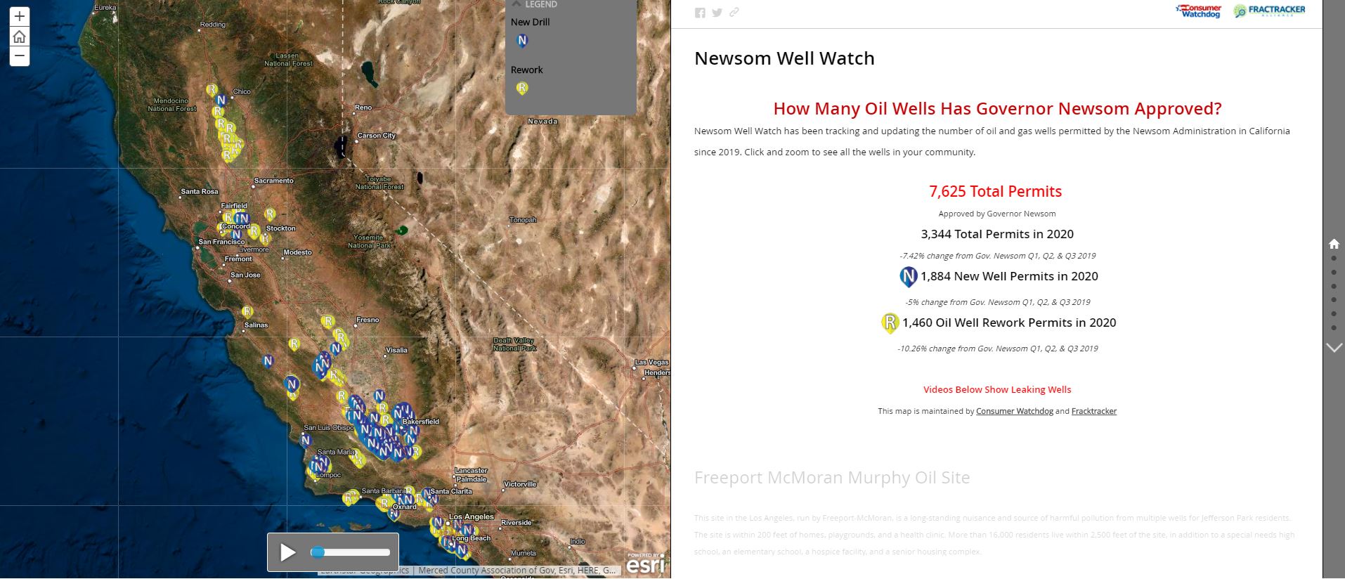
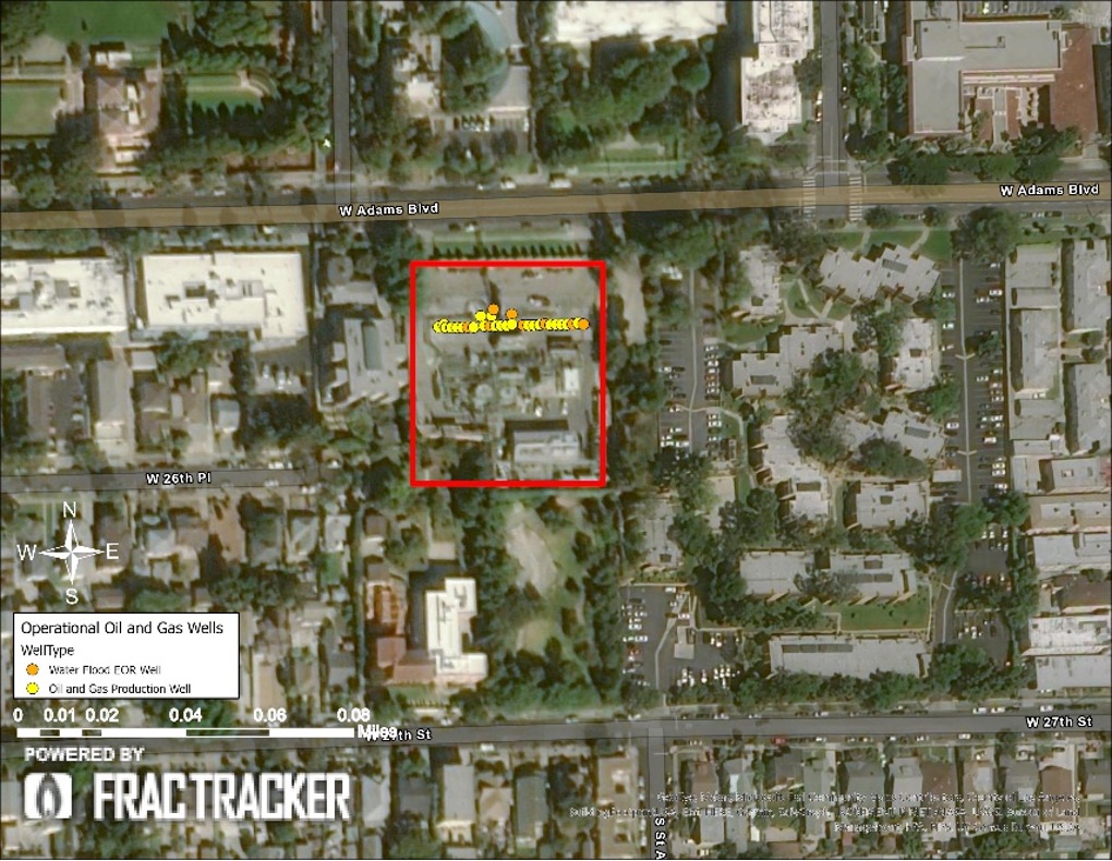
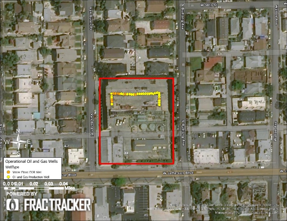
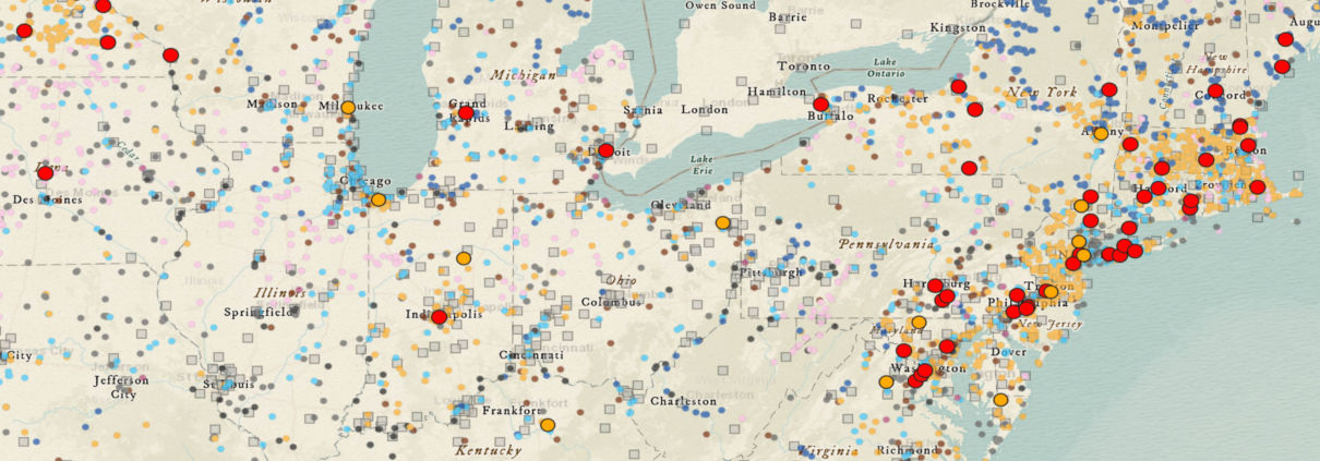
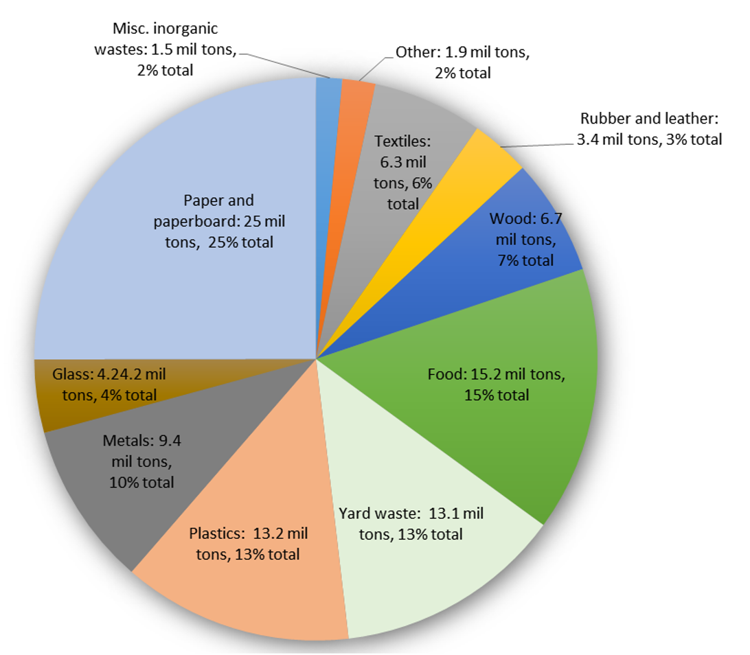
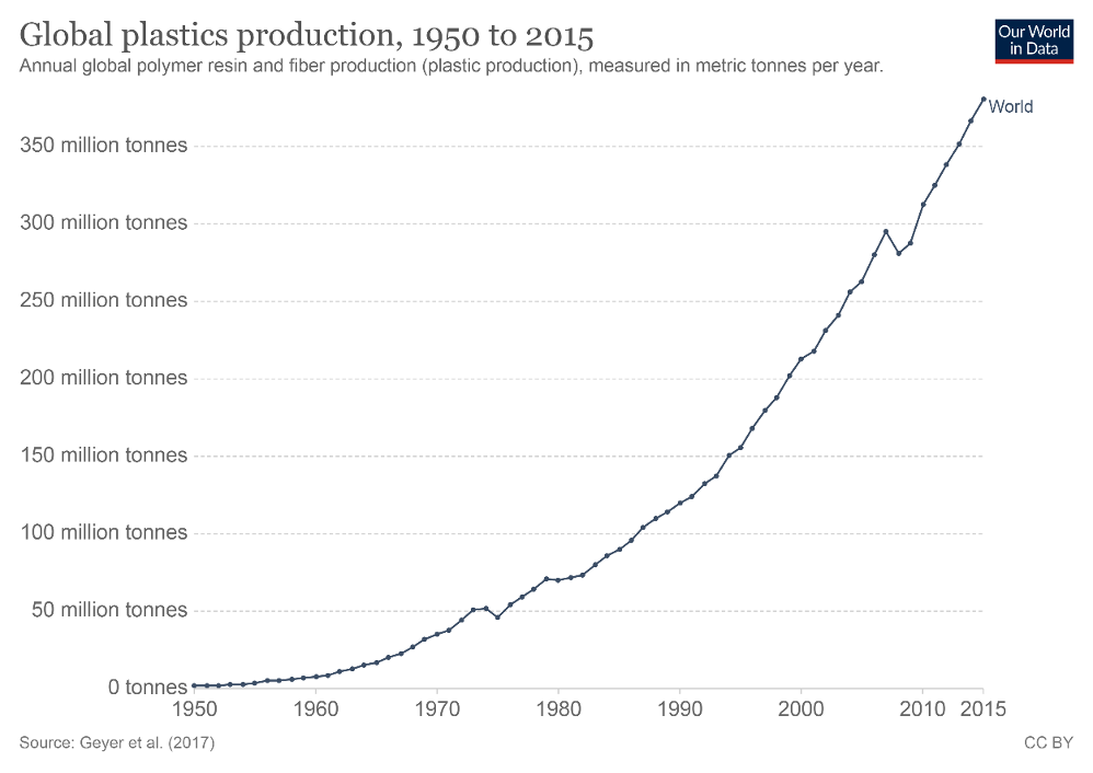
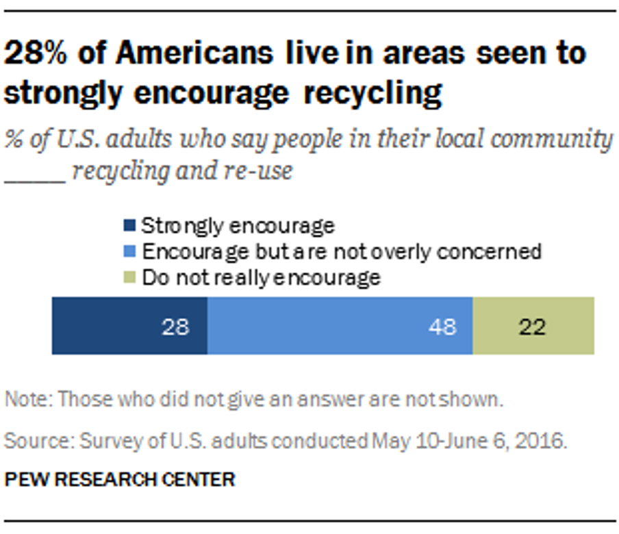
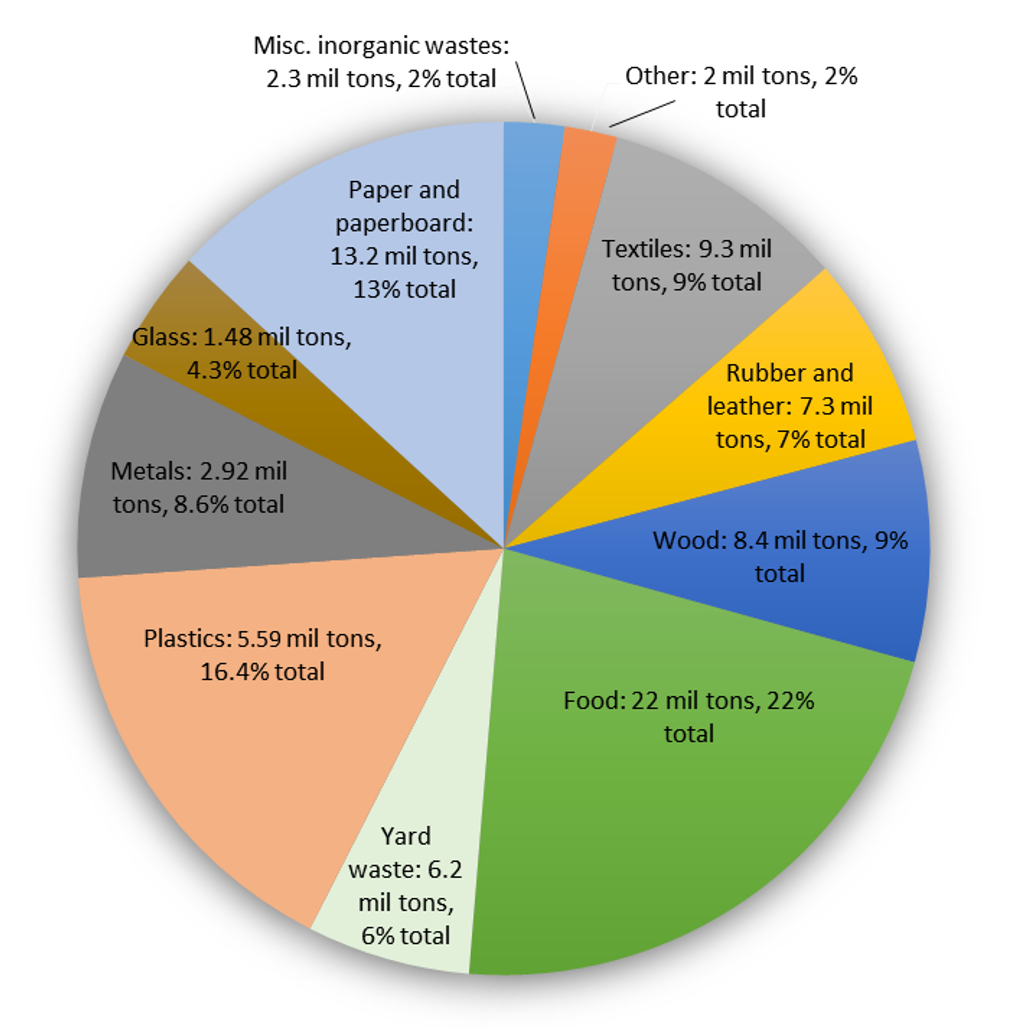
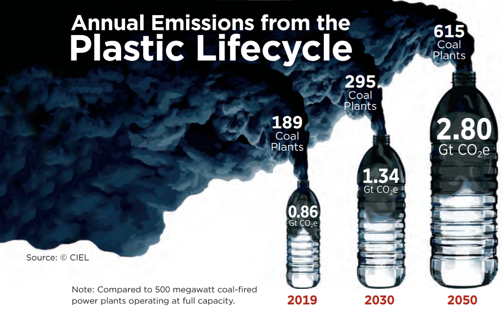


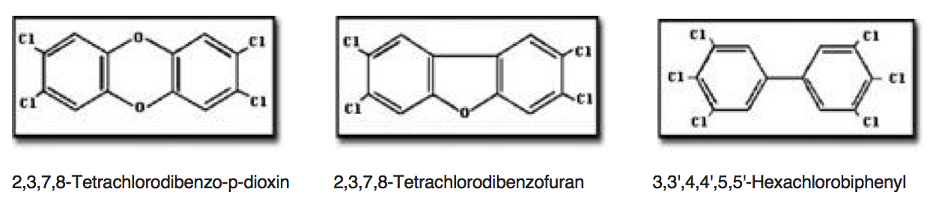
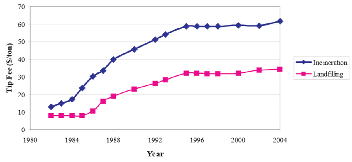
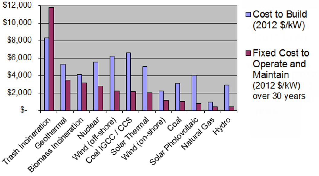
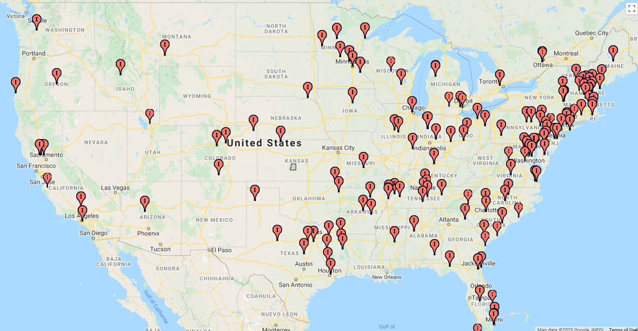
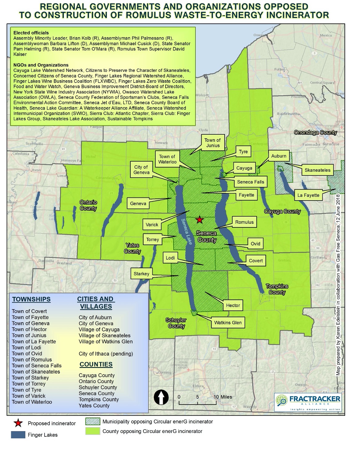
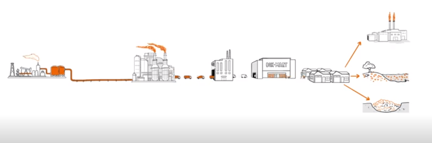
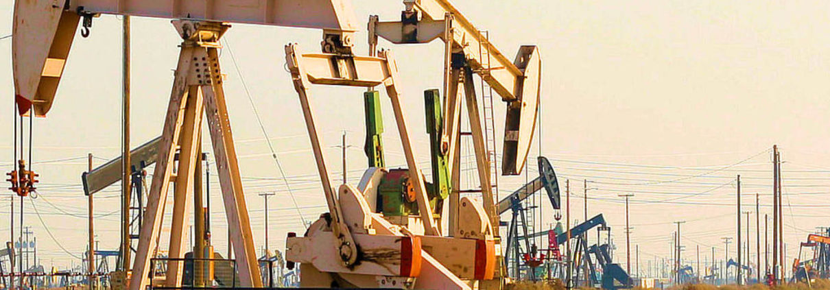

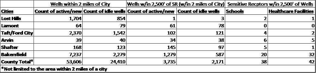
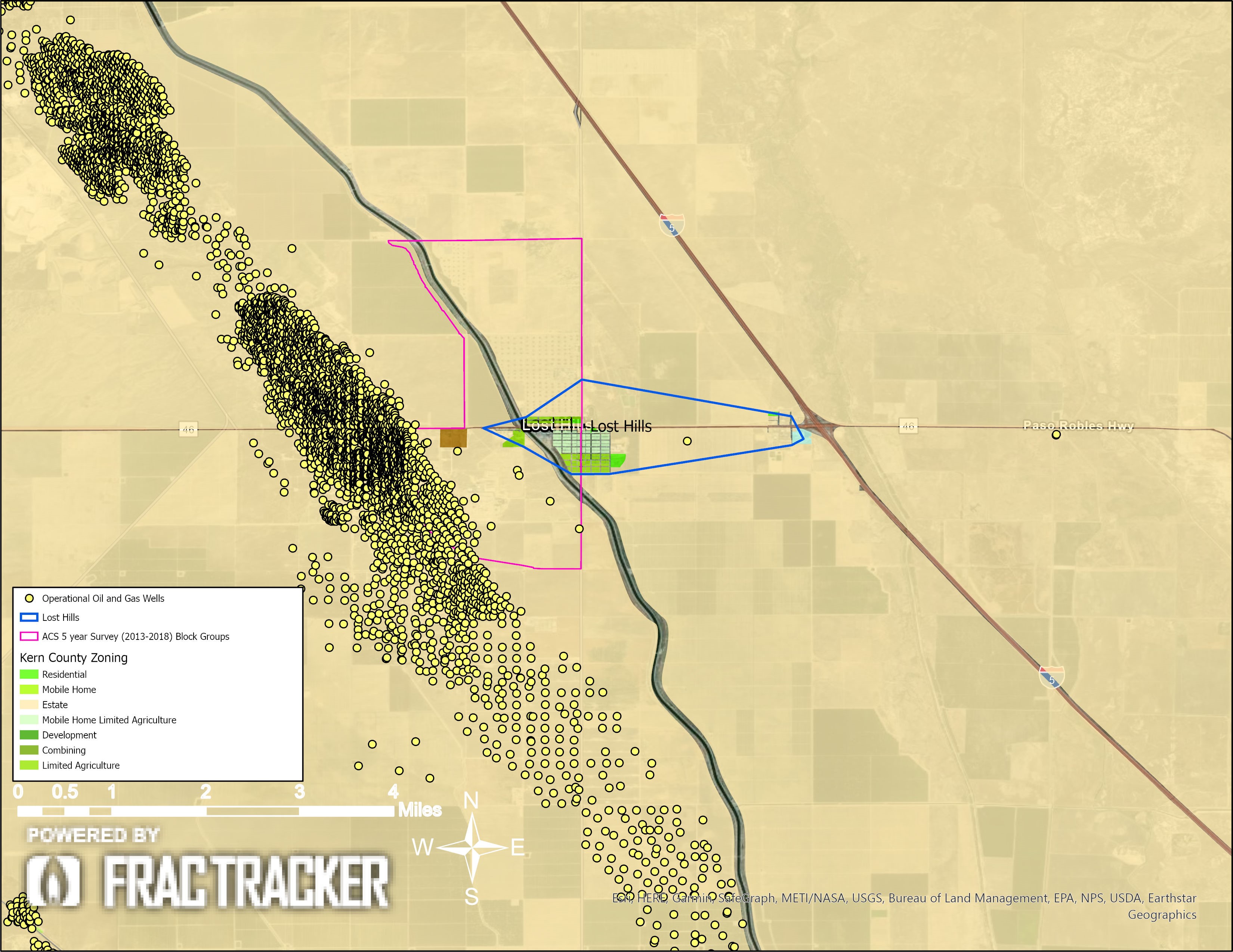
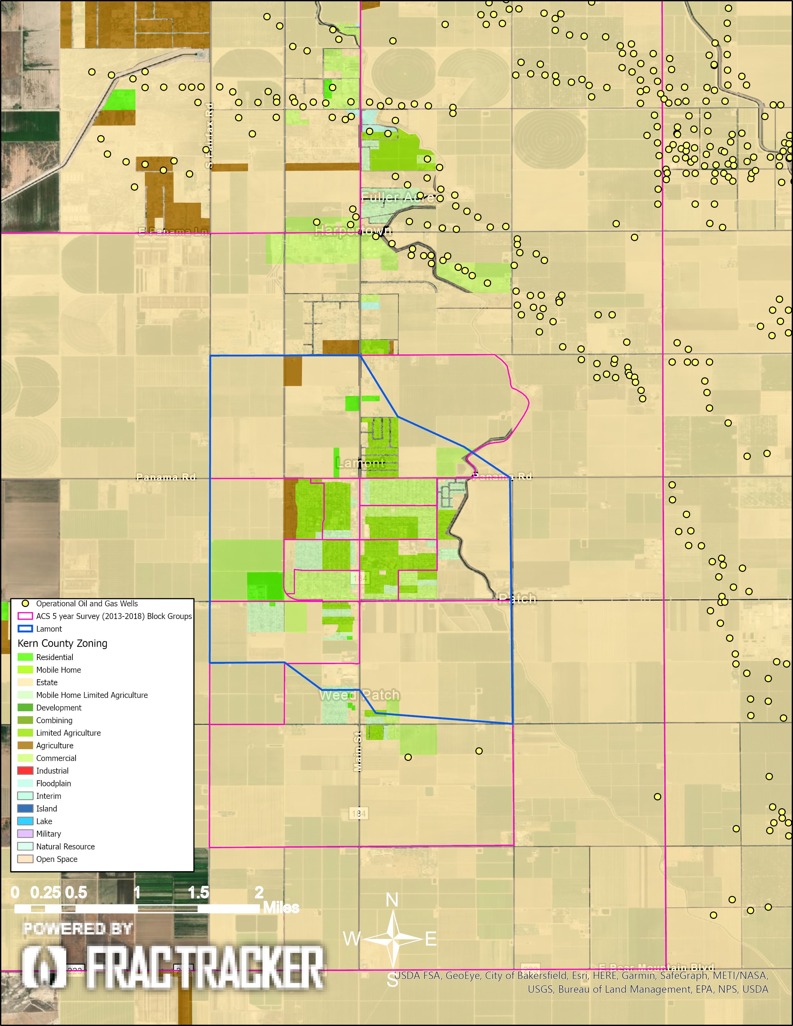
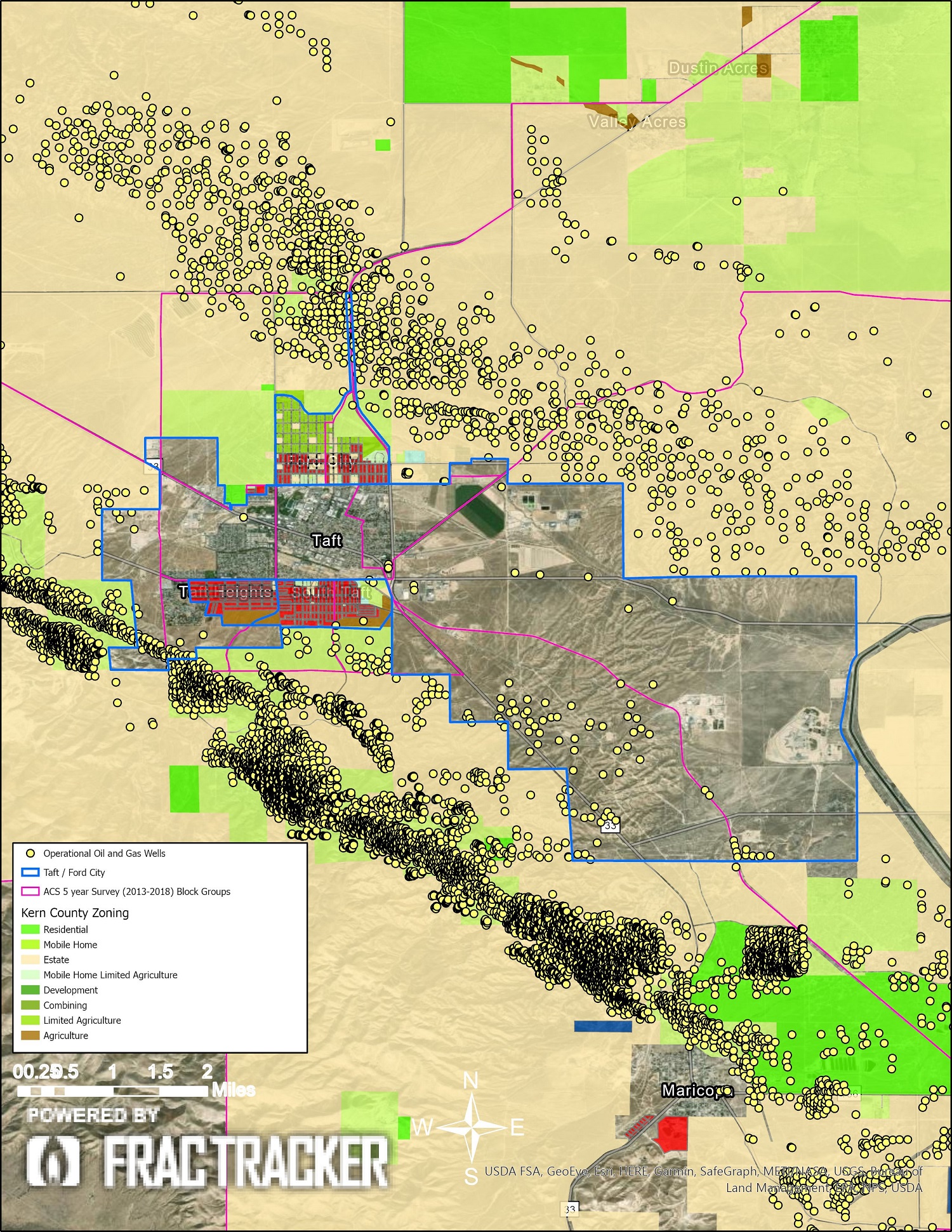
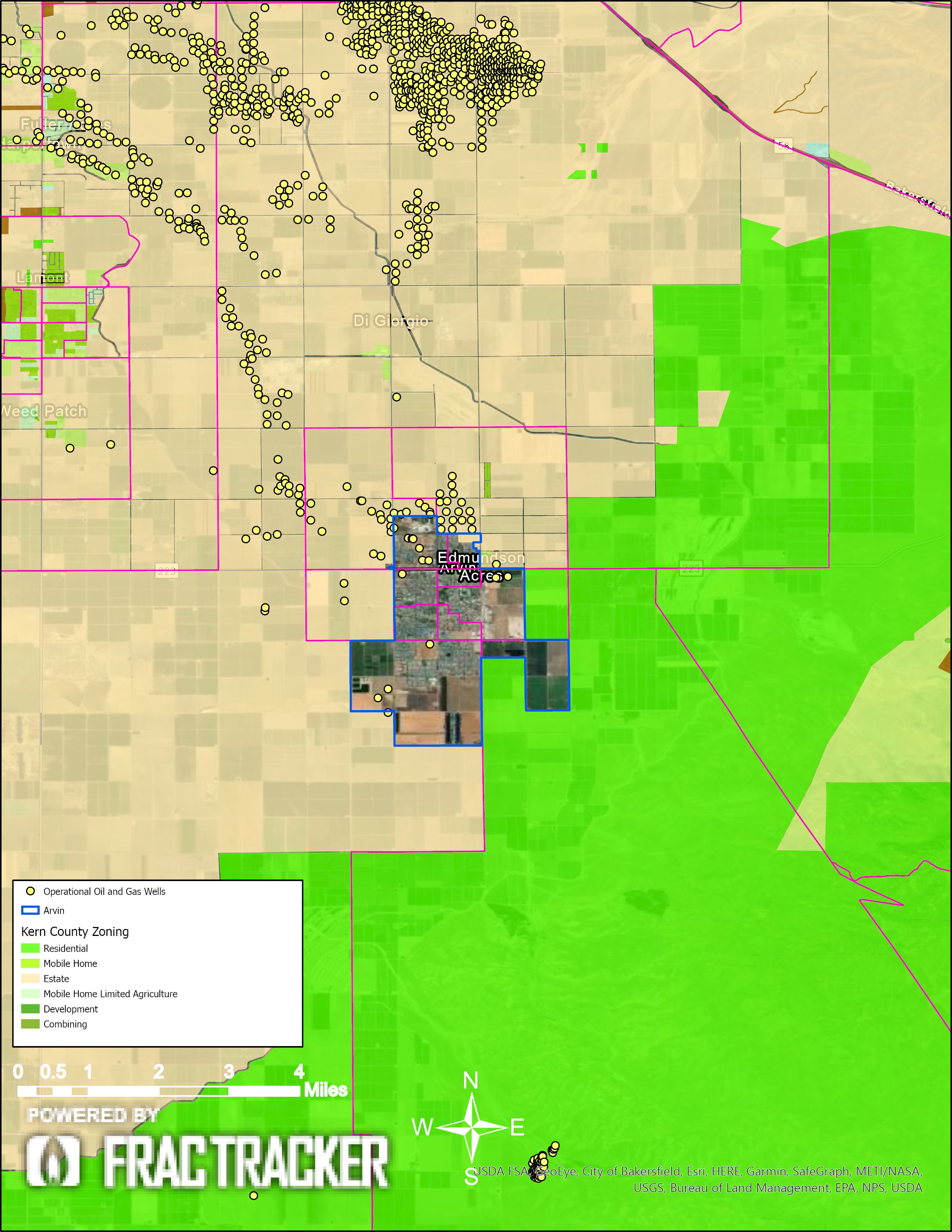
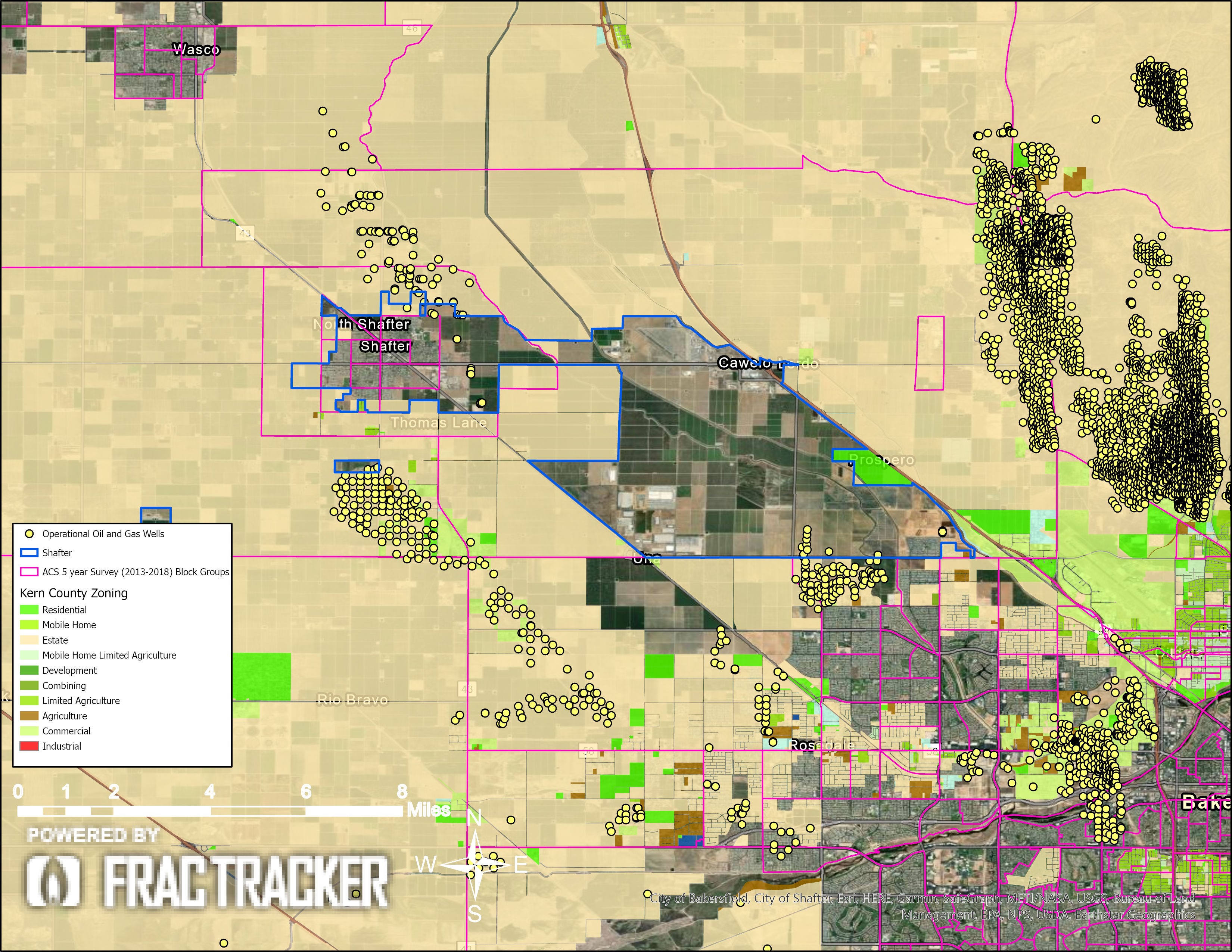
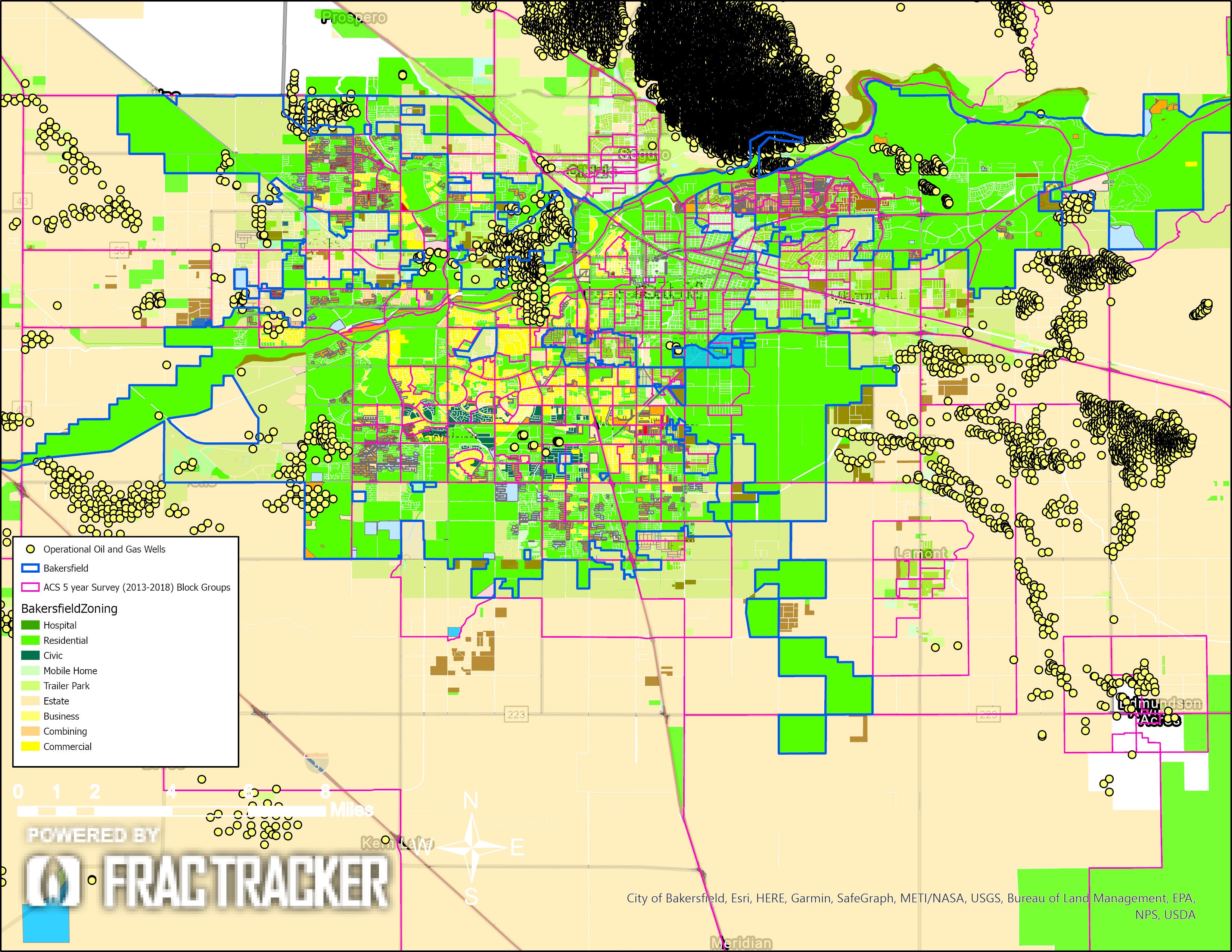

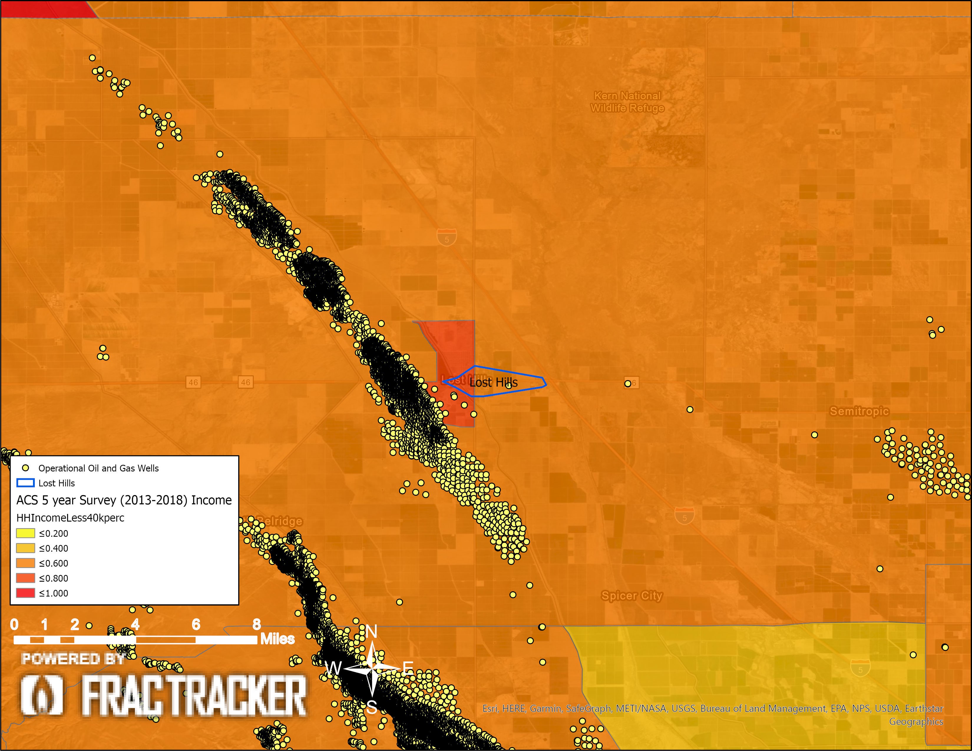
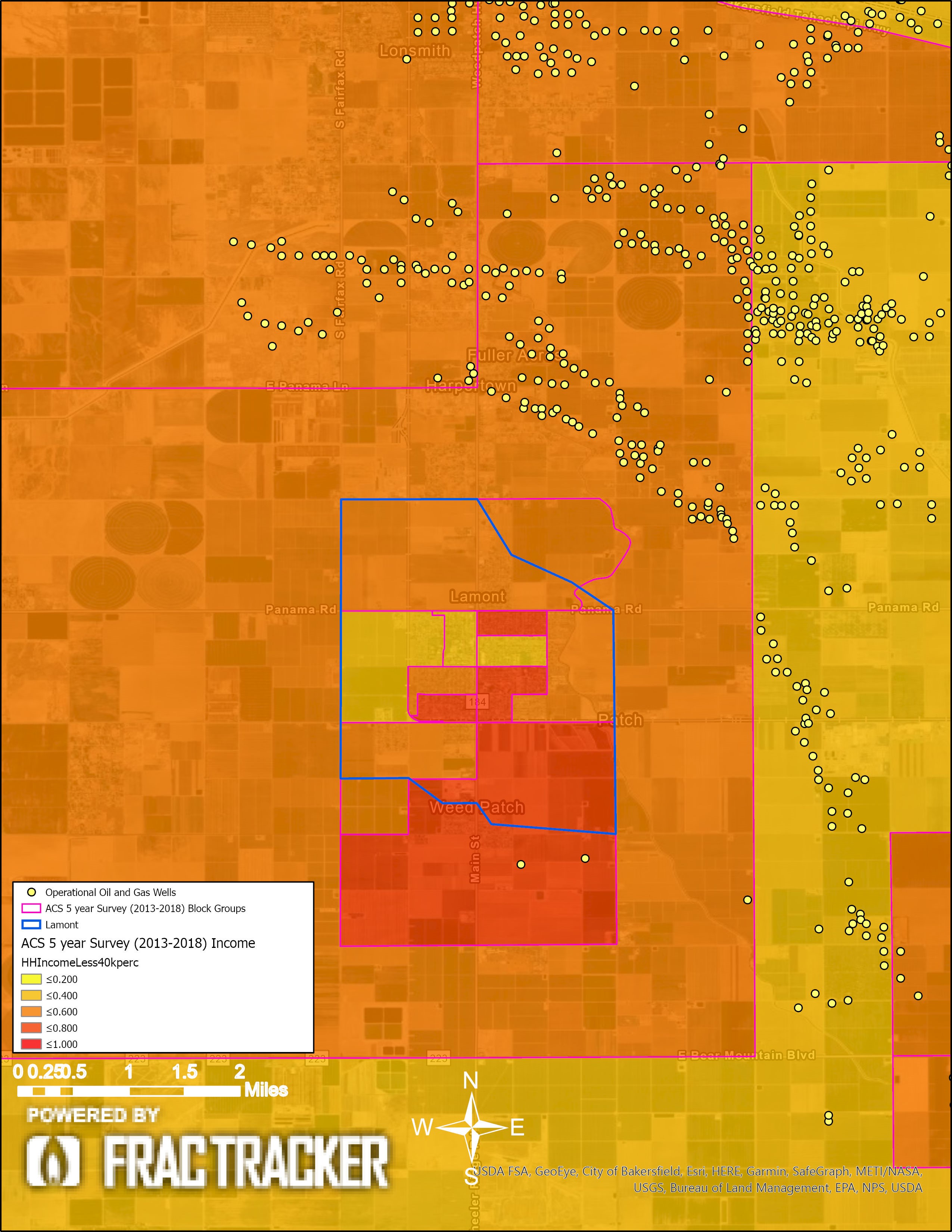
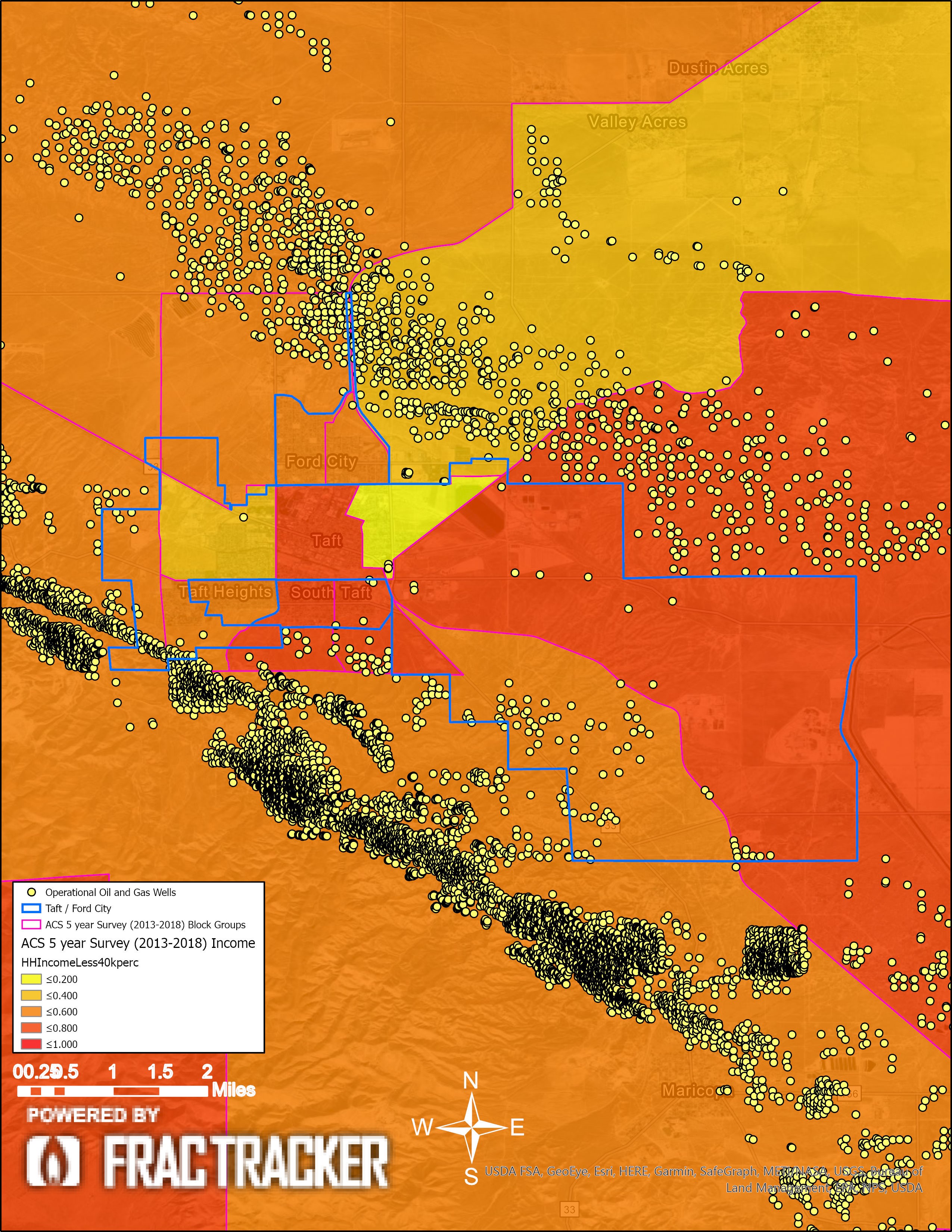
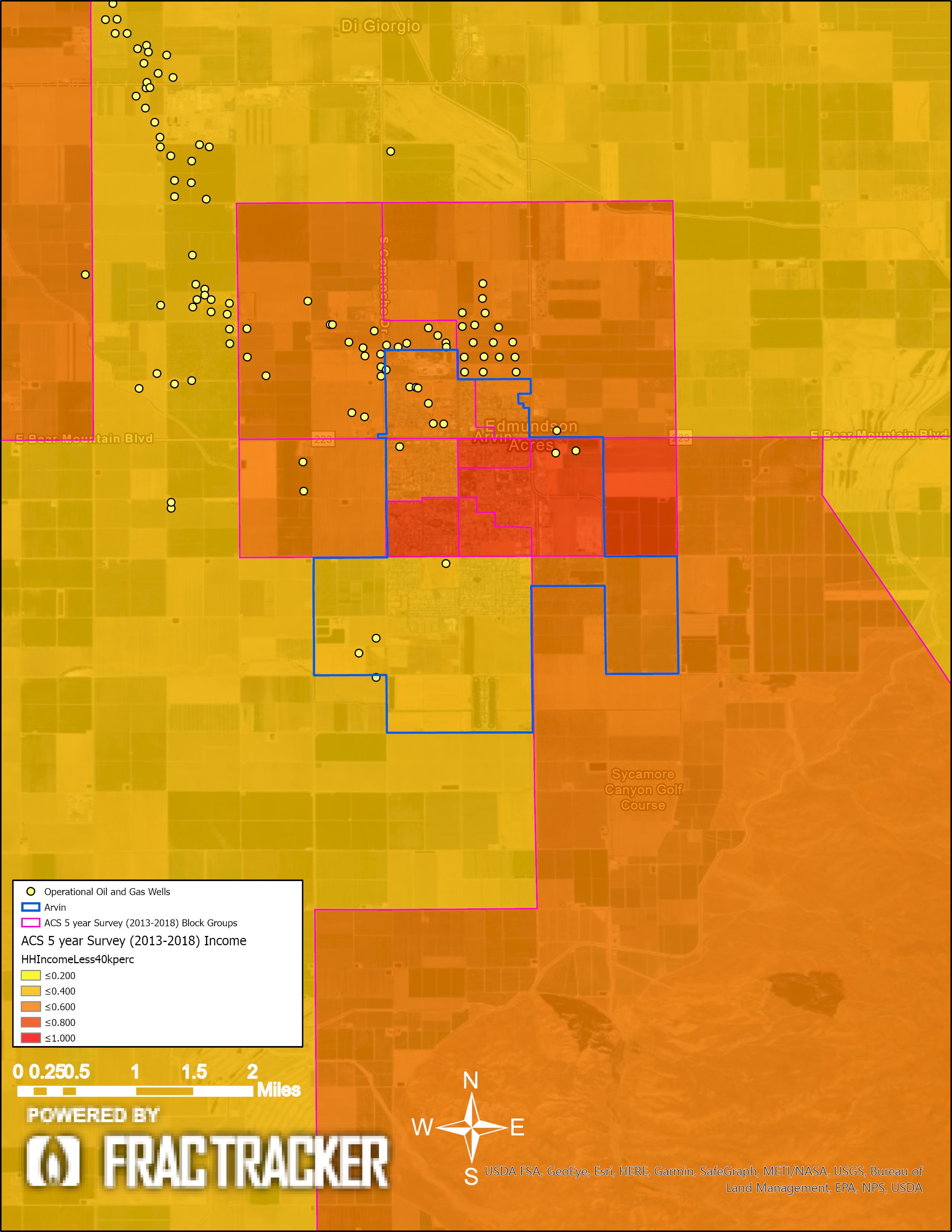
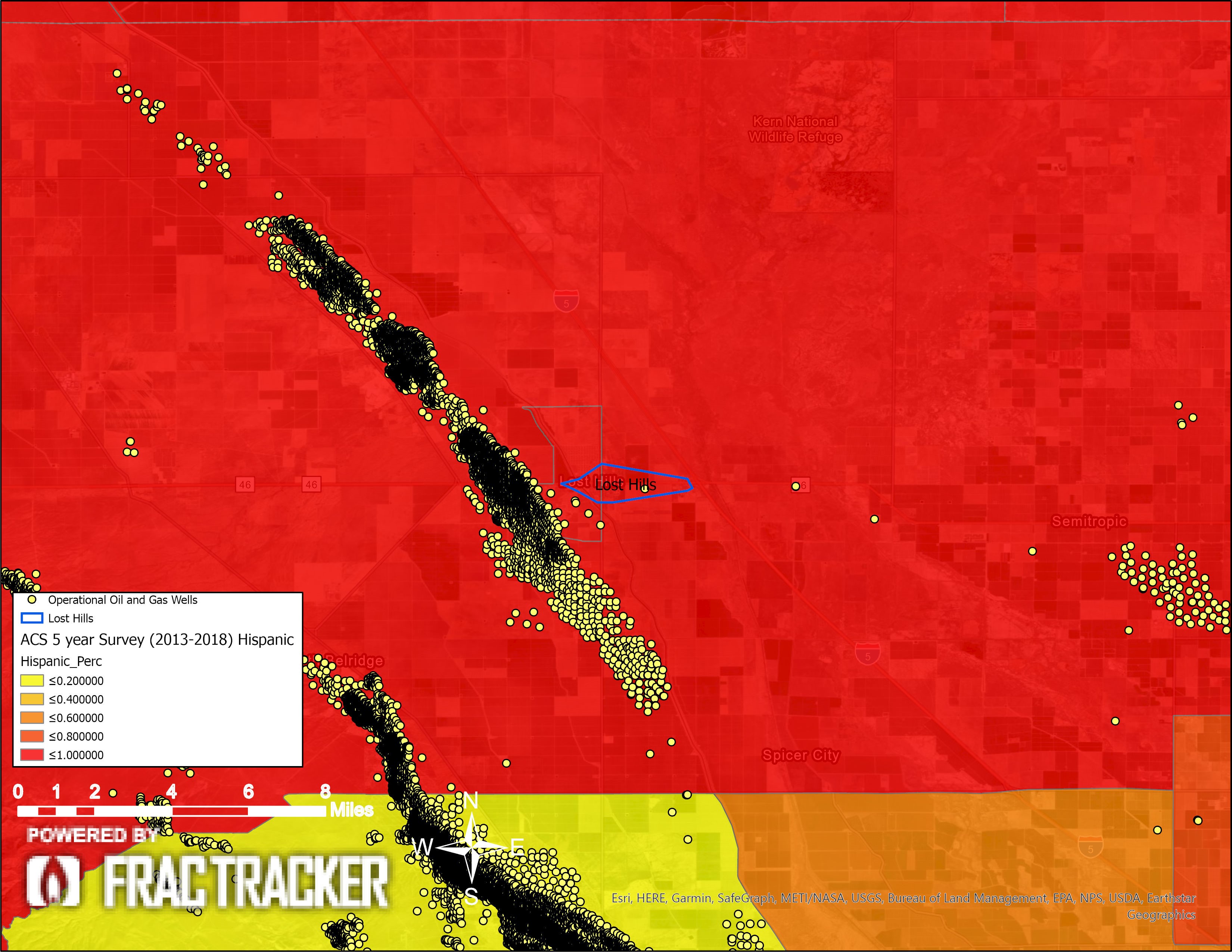
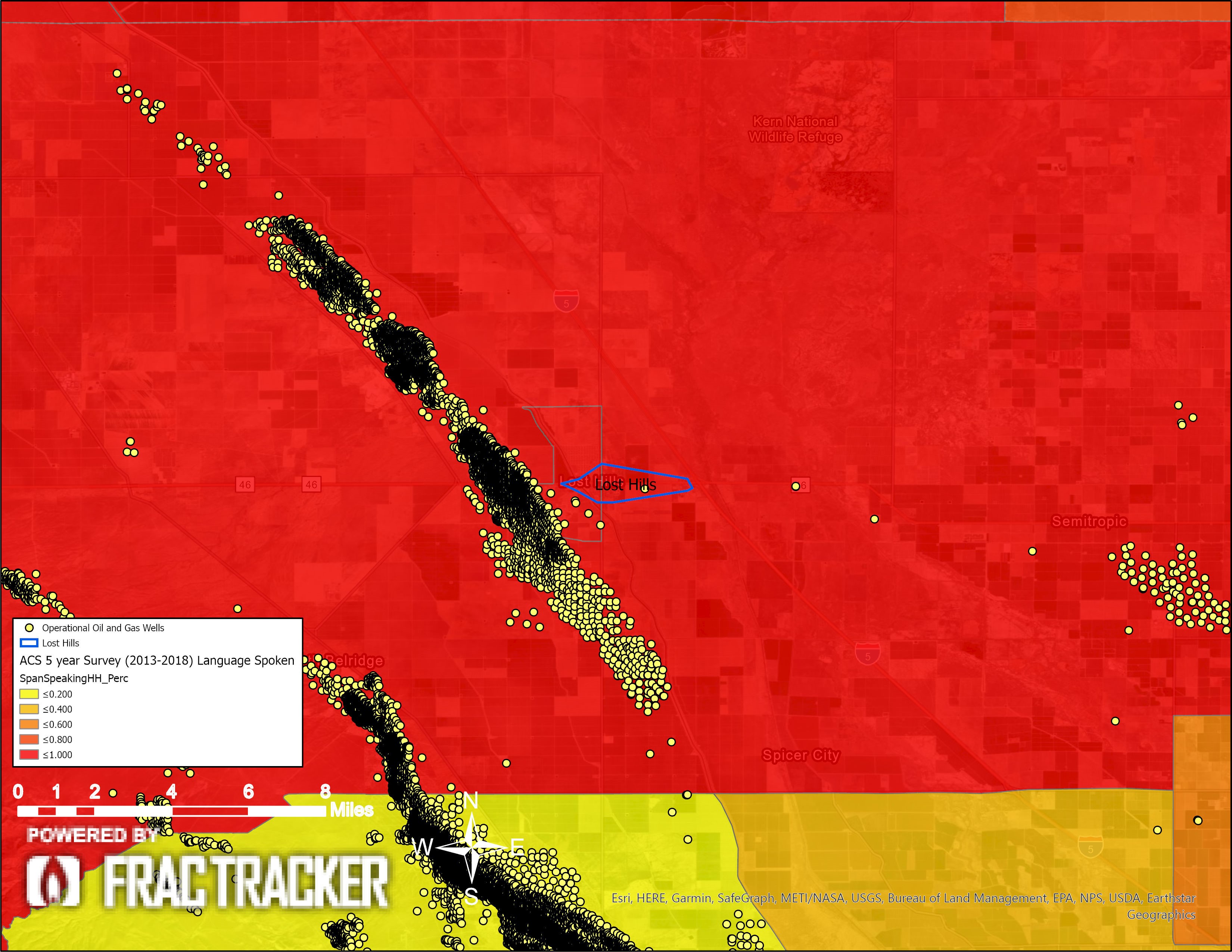
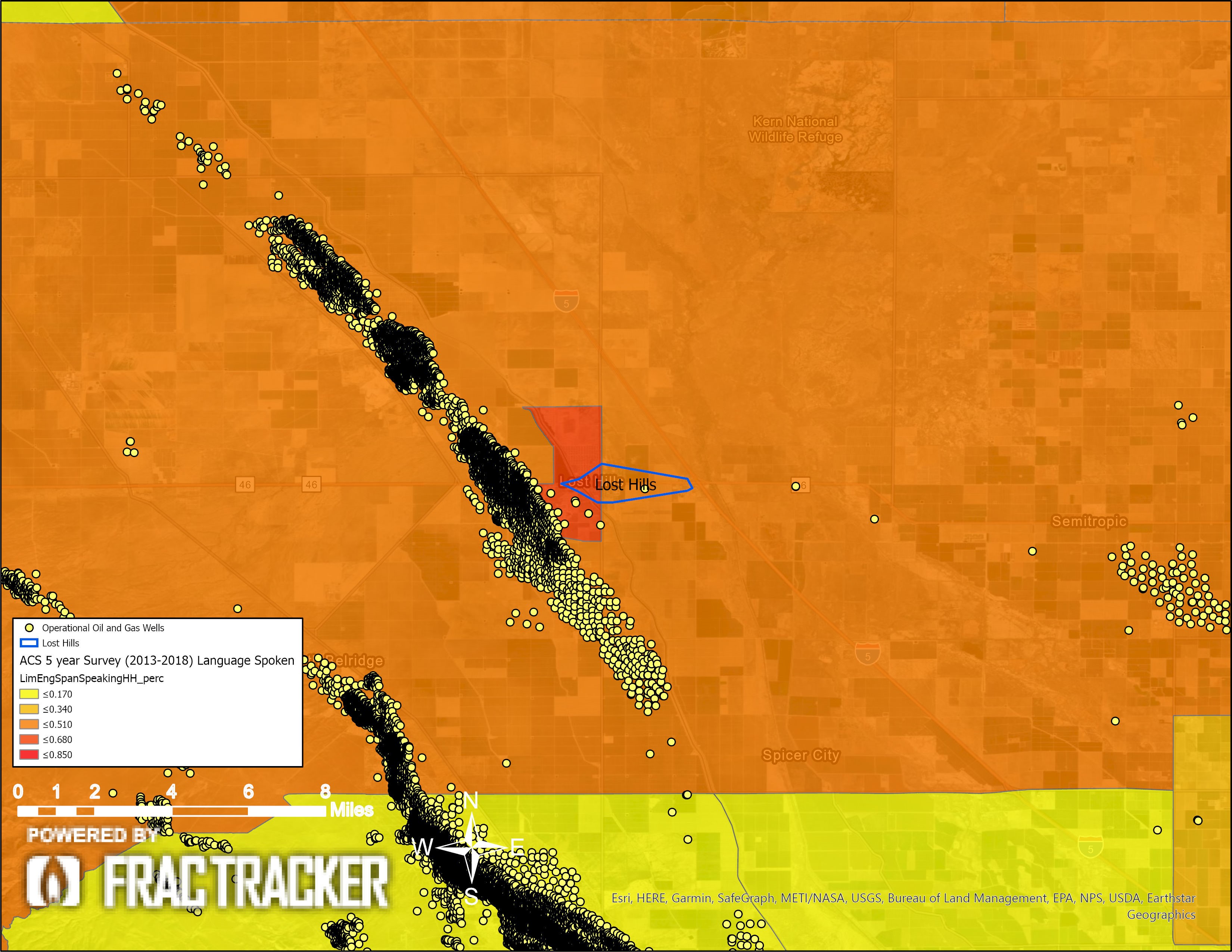
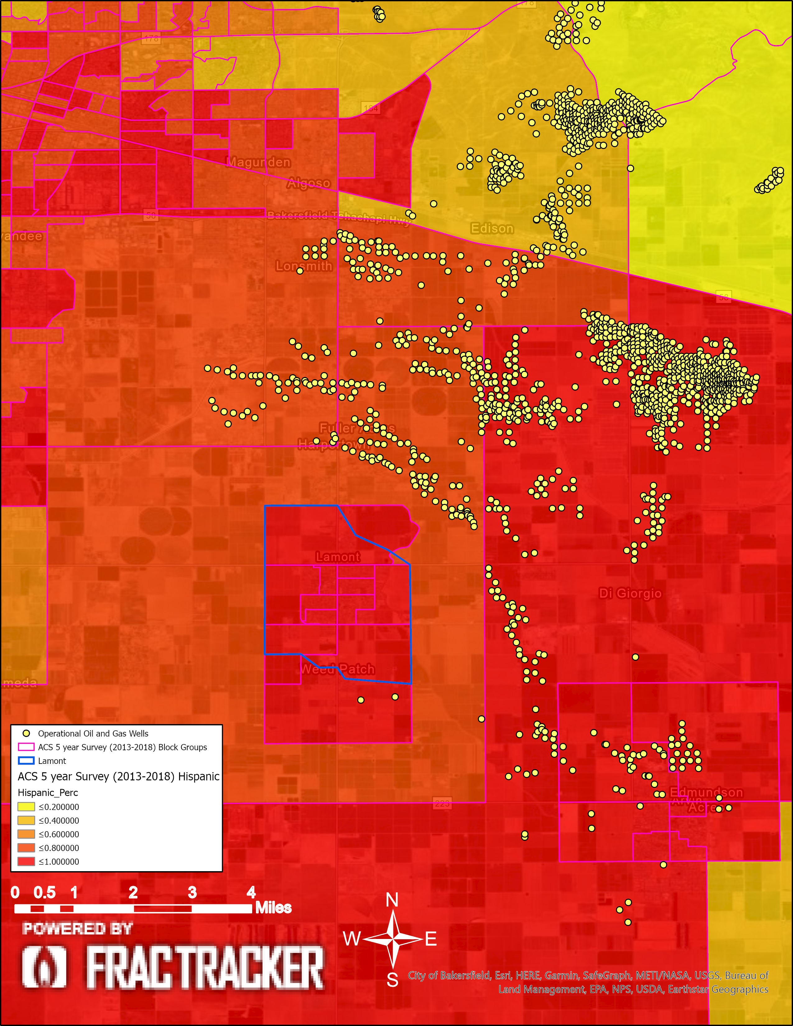
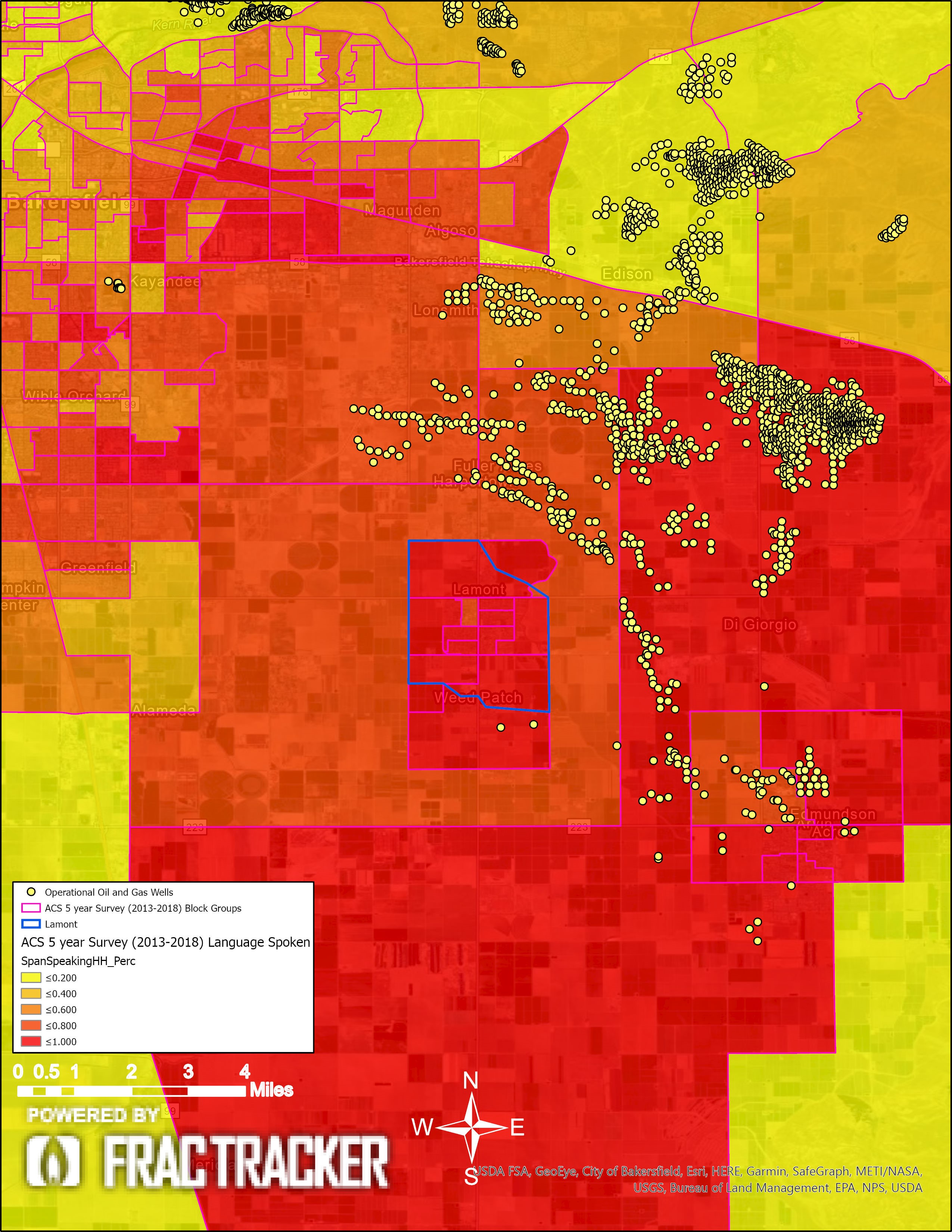
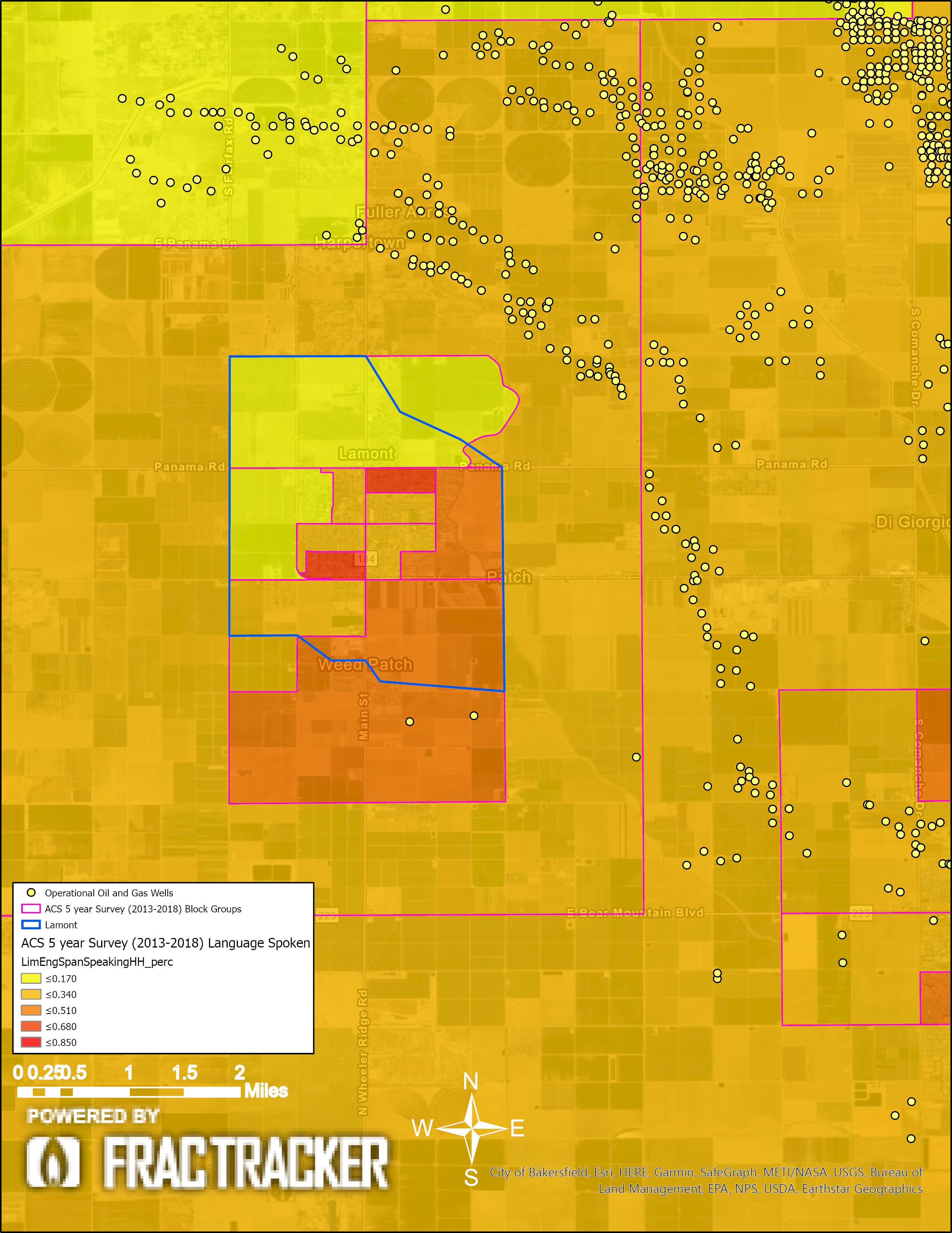
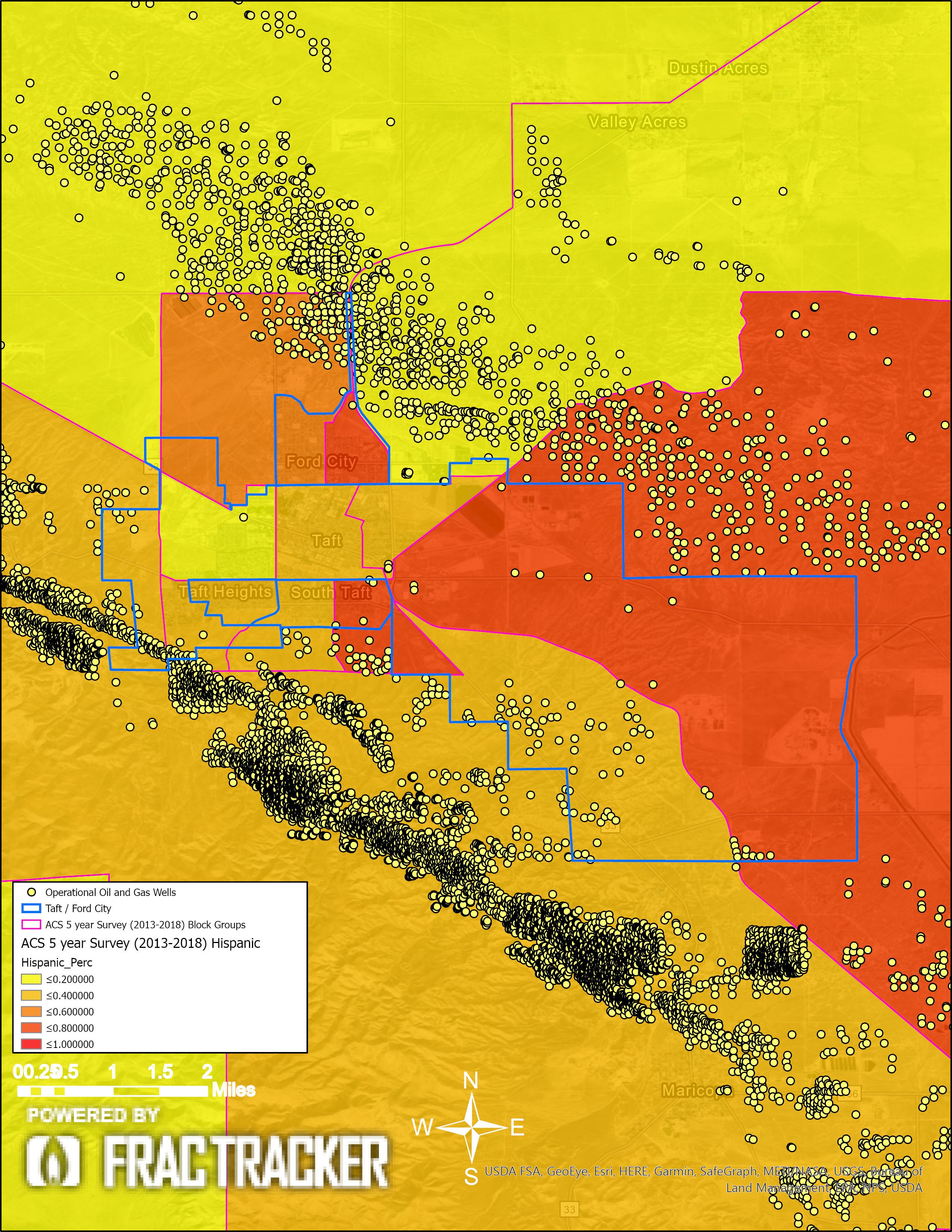
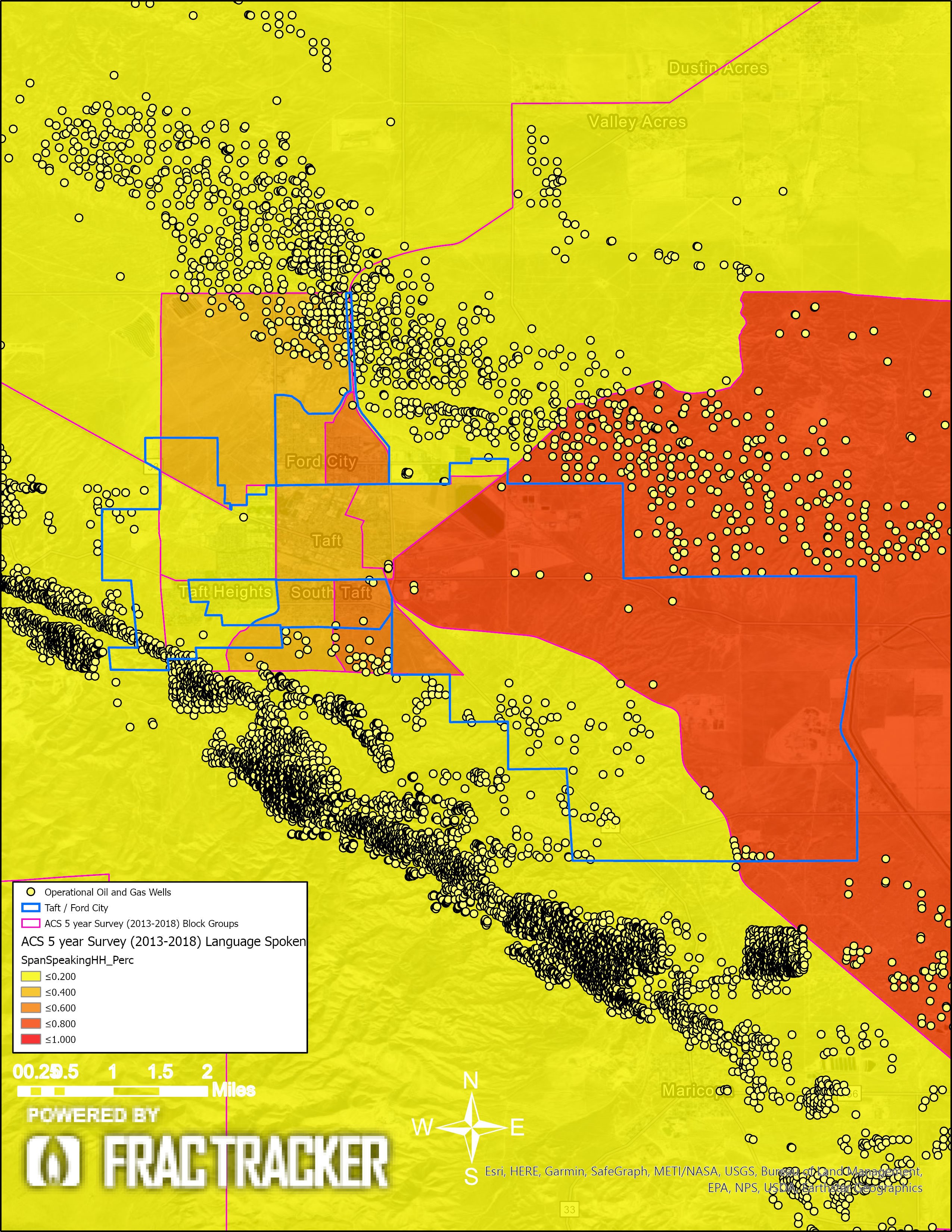
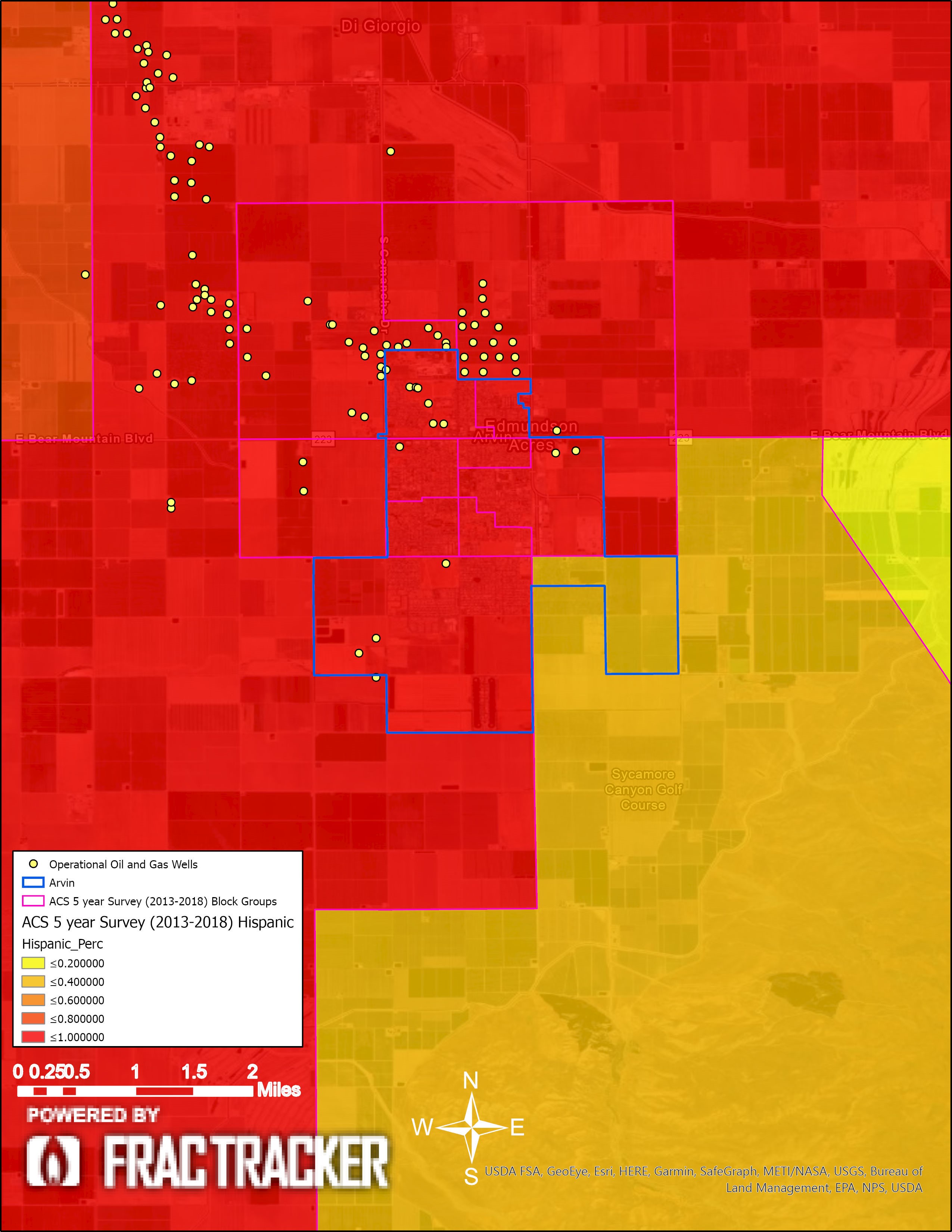
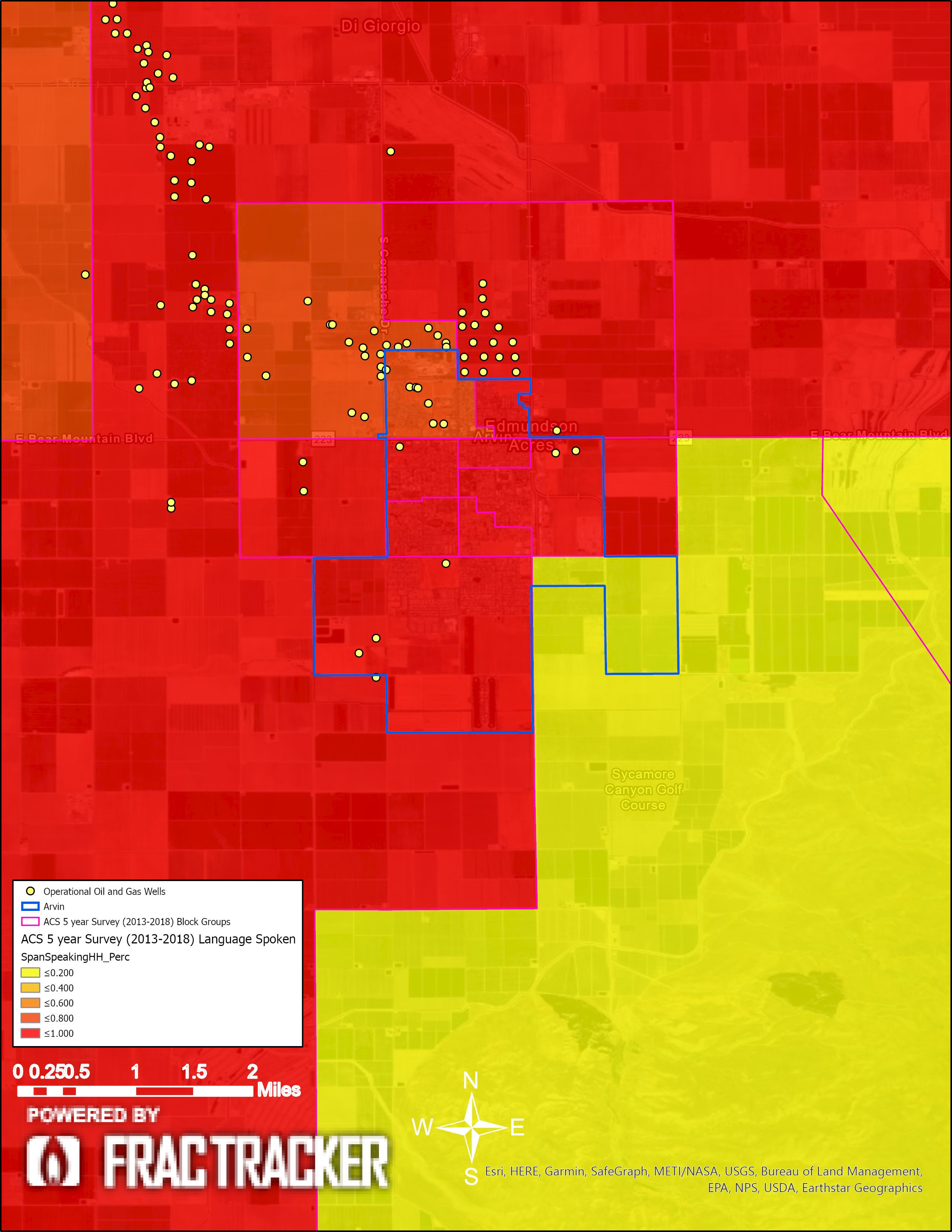
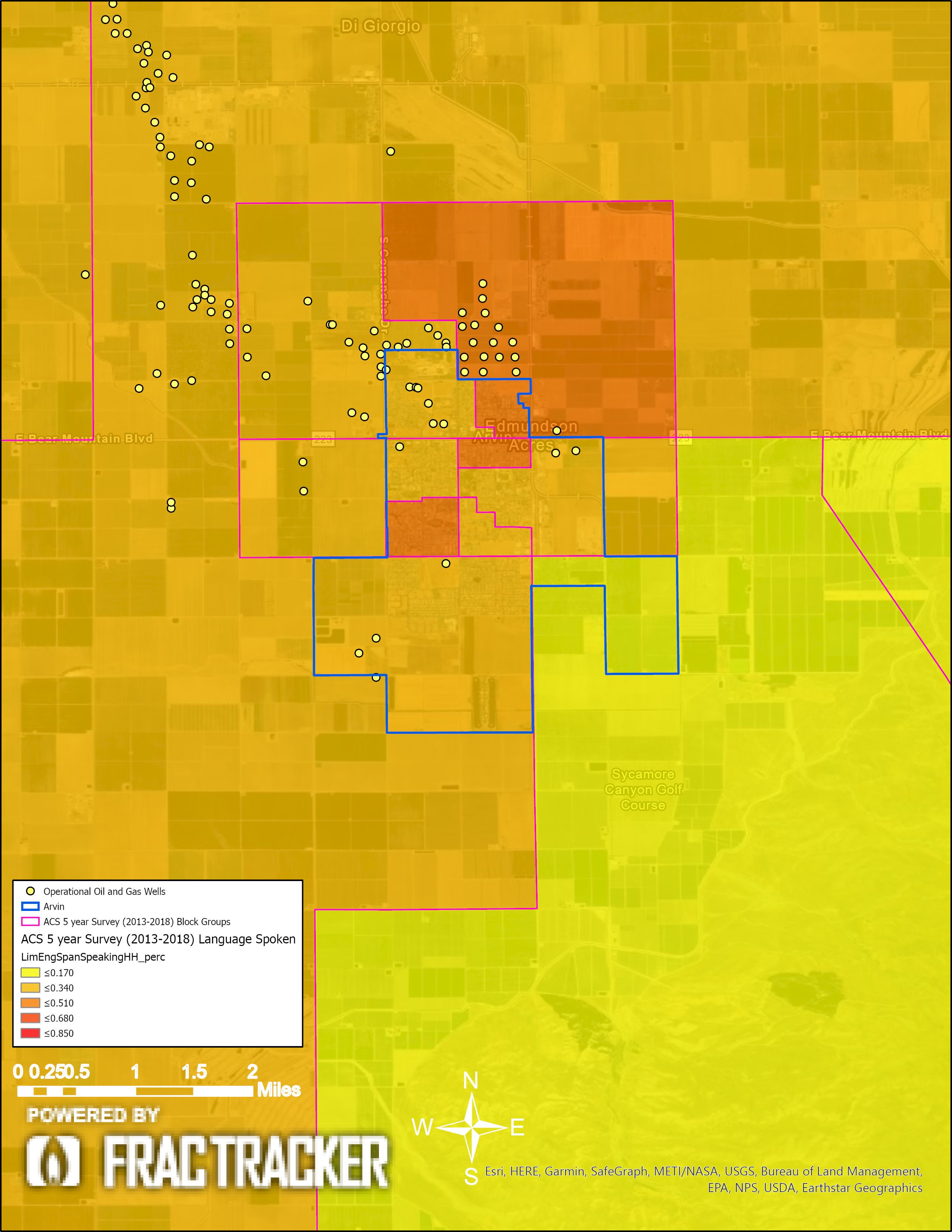
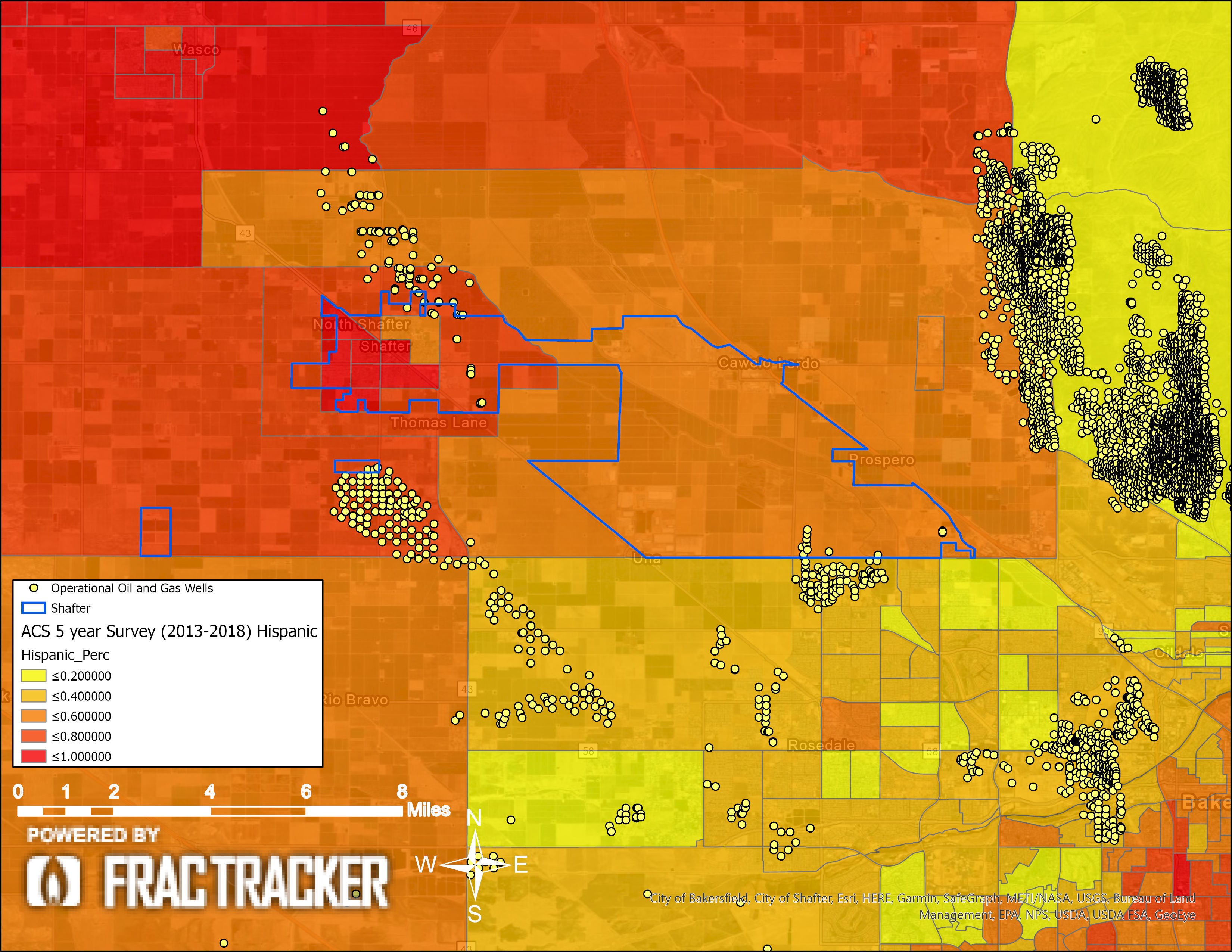
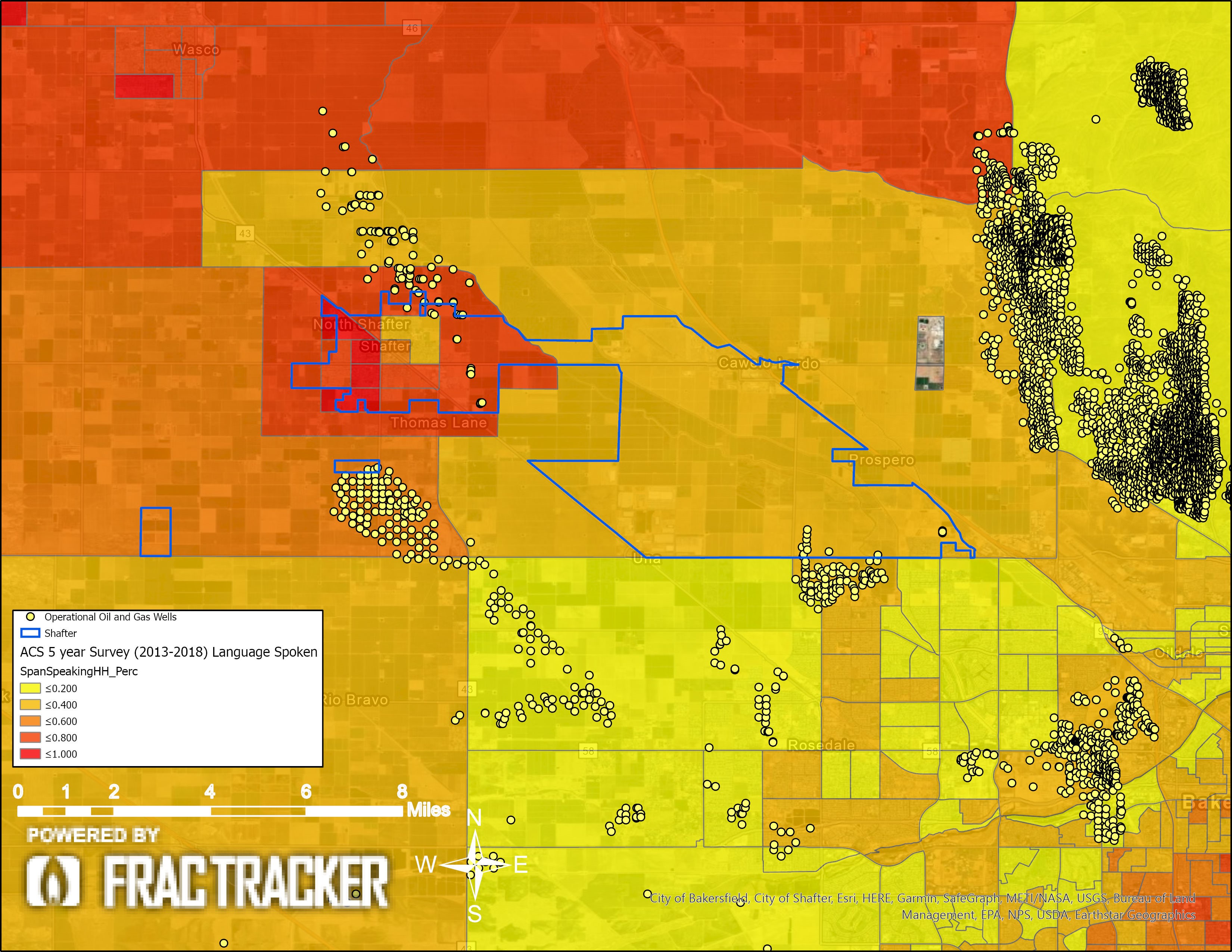
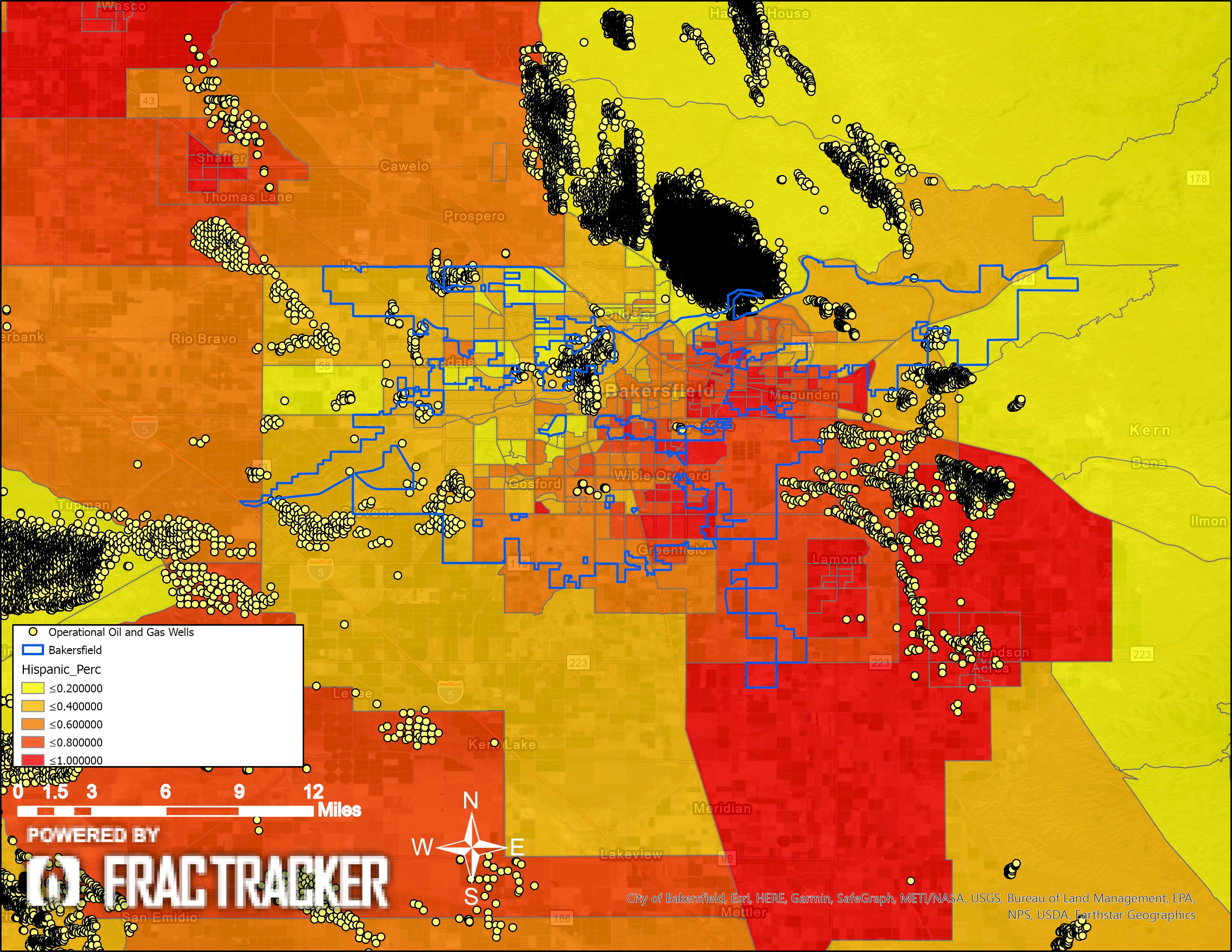
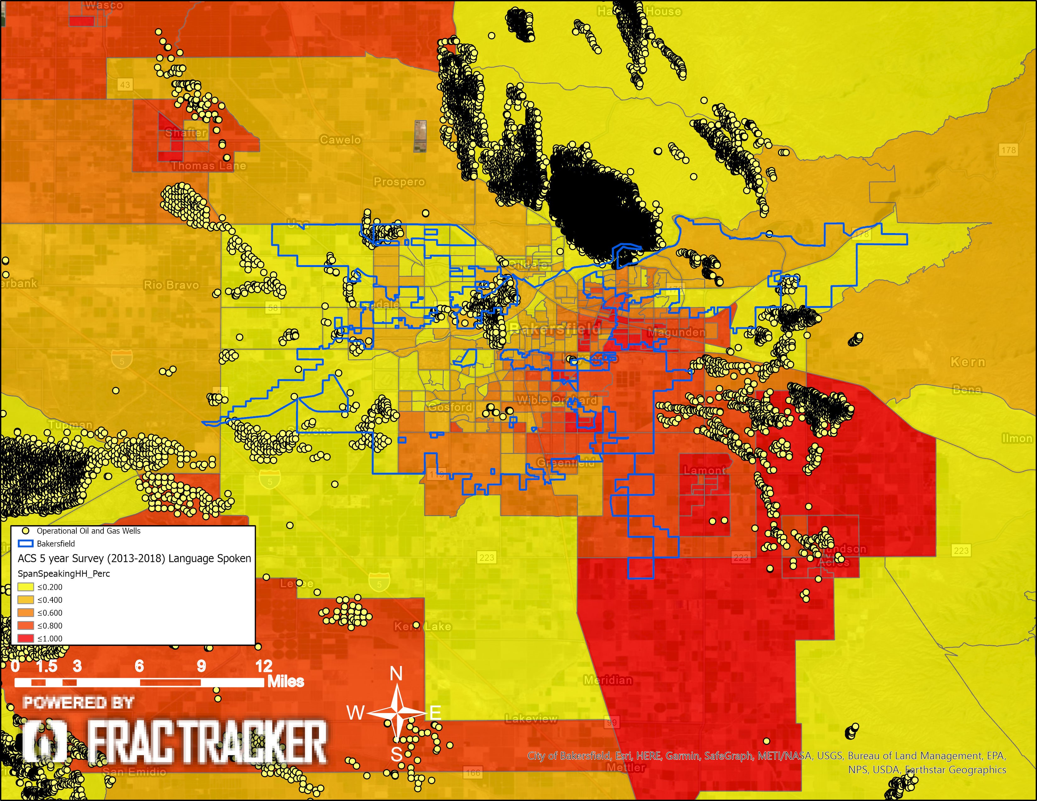
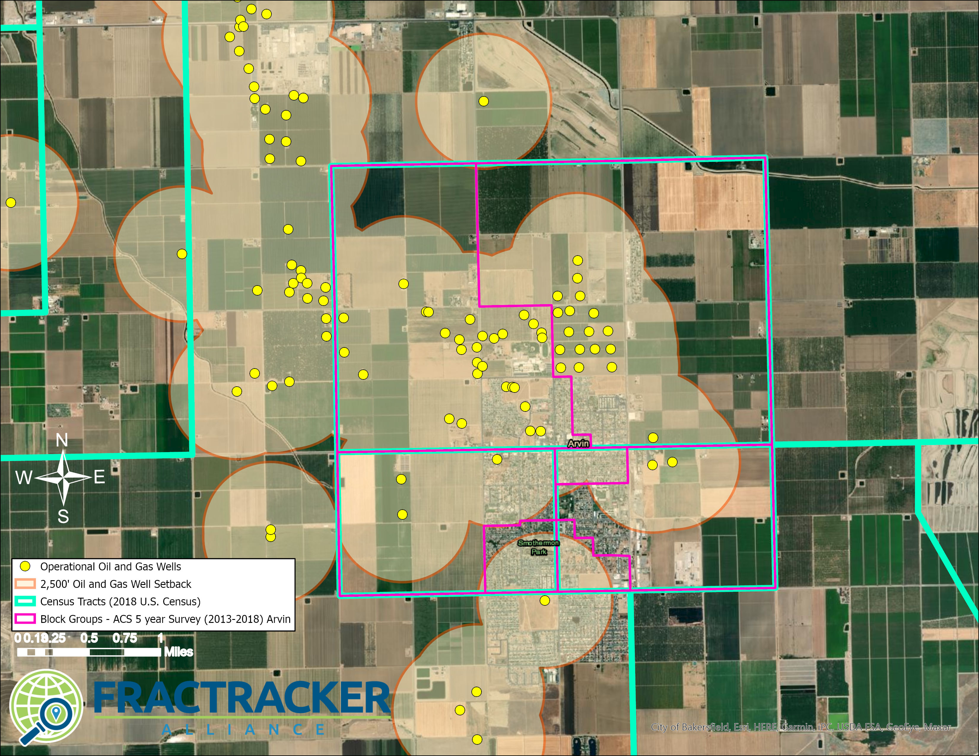
 Map A2. Shafter Census Designated Areas. The map shows the city of Shafter and includes both census tracts and census block groups for comparison. It shows operational oil and gas wells in the map, along with 2,500’ buffers. This Frontline Community would not be included in an analysis that only considers census tracts containing Tier 1 areas negatively impacted by oil and gas extraction operations. The census tract containing the North Shafter oil field forms a donut around the city of Shafter.
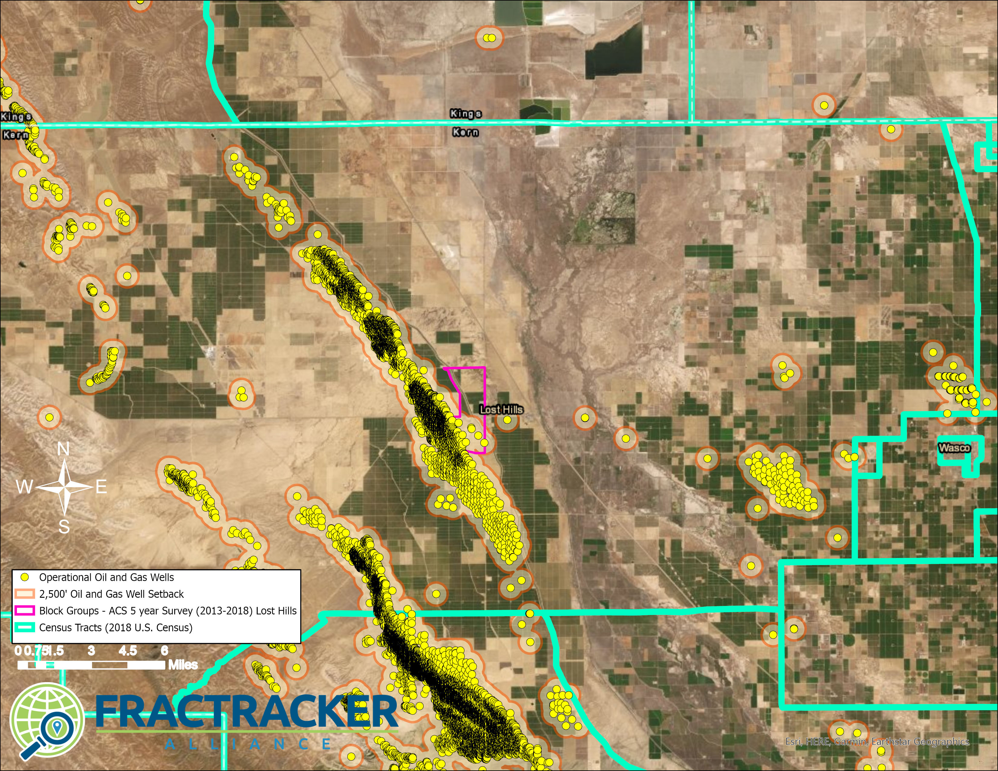
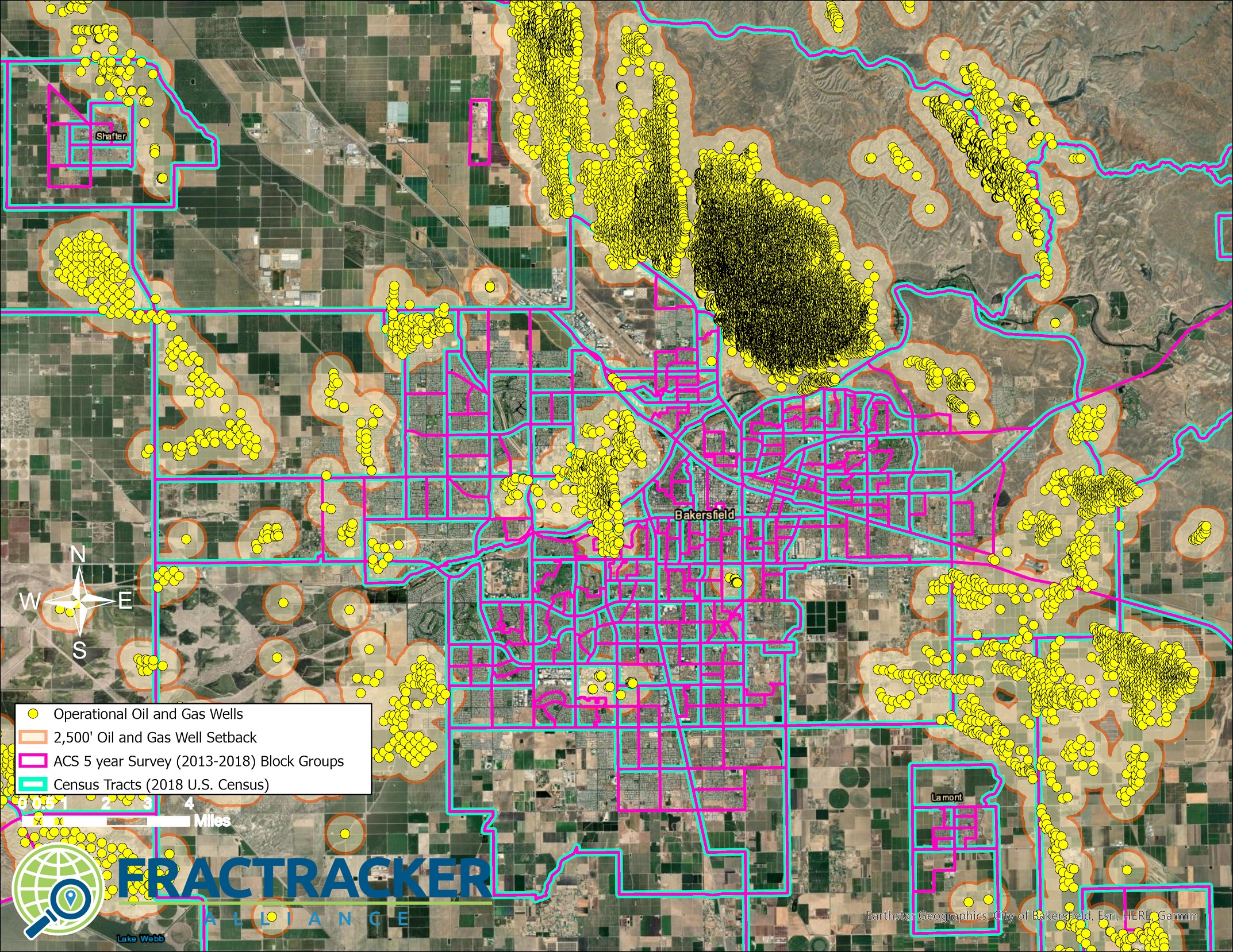
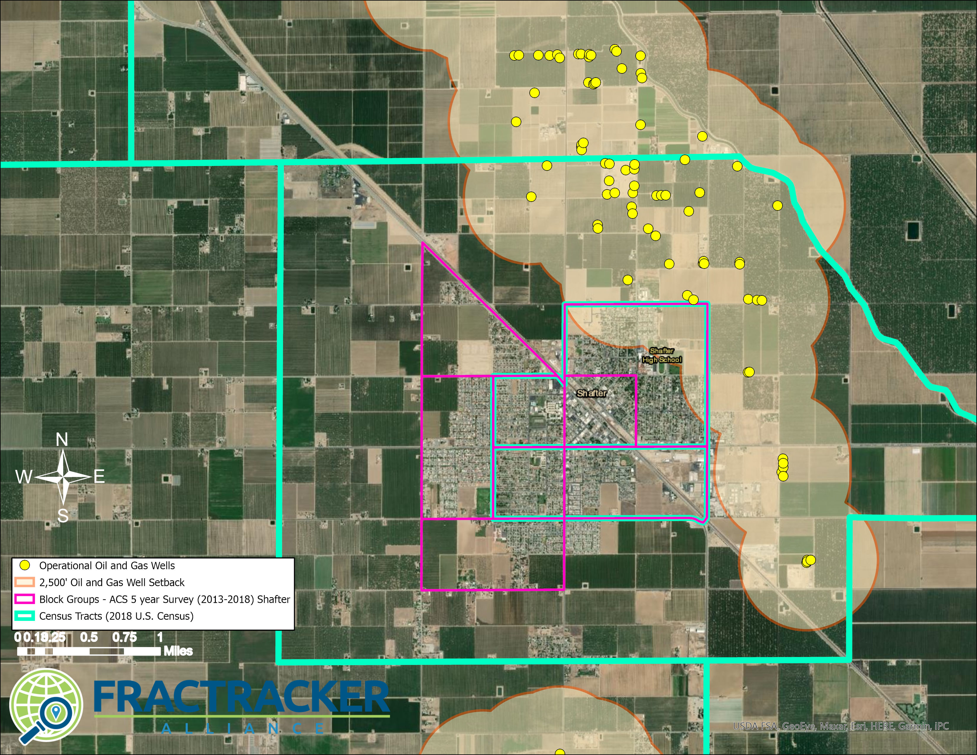
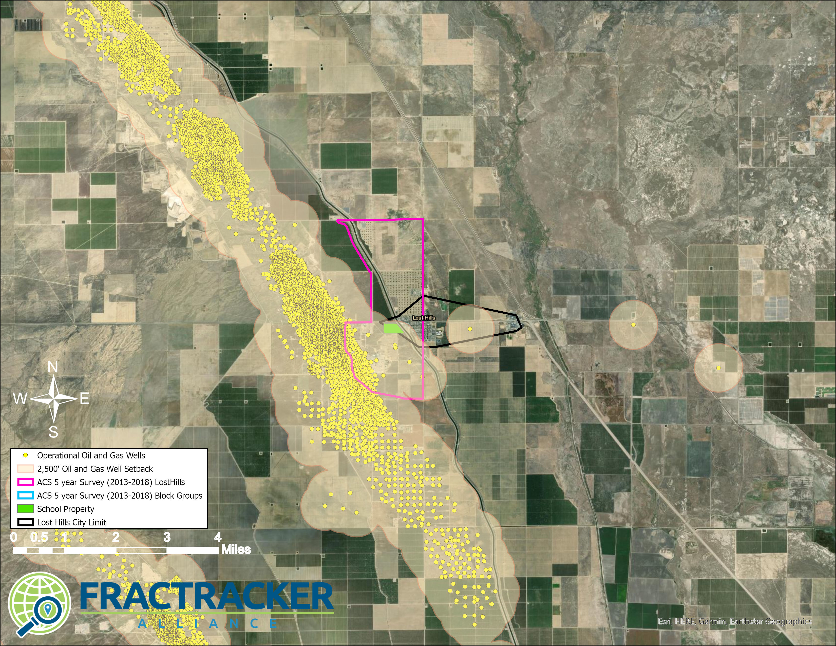
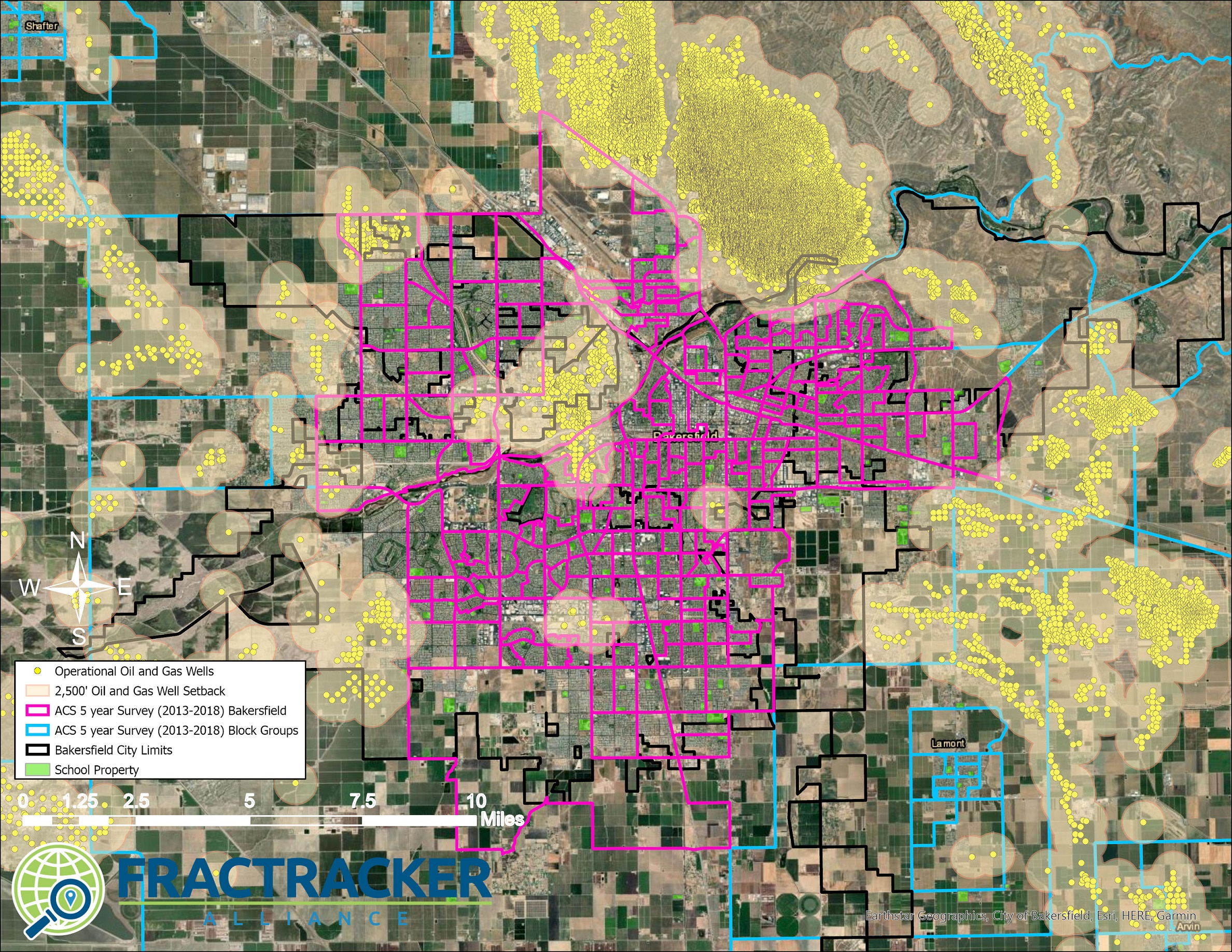
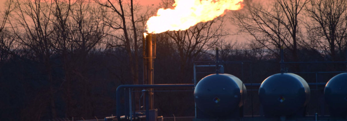 Ted Auch, FracTracker Alliance
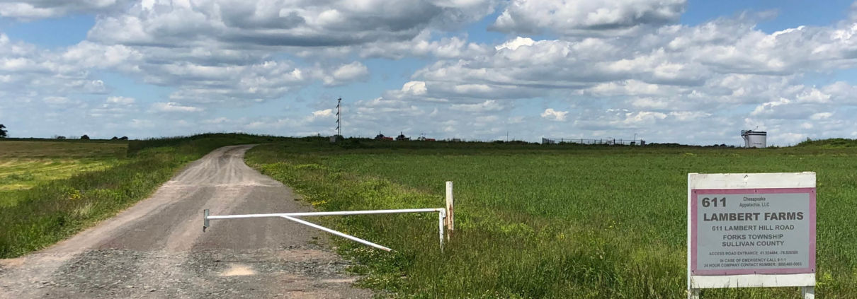
 Photo by Ted Auch, FracTracker Alliance, with aerial support by LightHawk