Data and Analysis Archives - Page 10 of 22

Land-Use Change, the Utica Shale, and the Loss of Ecosystem Services

May 16, 2013/by Ted Auch, PhD

By Ted Auch, PhD – Ohio Program Coordinator, FracTracker Alliance

In Ohio, Utica Well pads range in size from 5-15 acres. (Estimates for pipeline and retention ponds are unavailable.) That figure gives us the chance to estimate how hydraulic fracturing influenced changes to land-use, ecosystem services, plant productivity, and soil carbon loss.

Working with Caleb Gallemore and his Ohio State University GIS class, we created a data set that estimated the percent cover for each well pad prior to drilling using the USGS and Department of Interior’s 2006 National Land Cover Database (NLCD, 2006) [1].

Figure 1. Ohio’s original vegetation cover and Utica Well permits as of April 30th, 2013

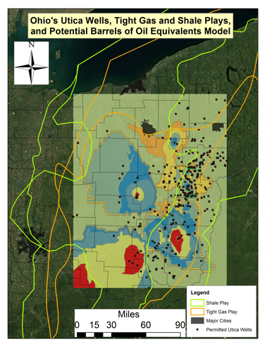
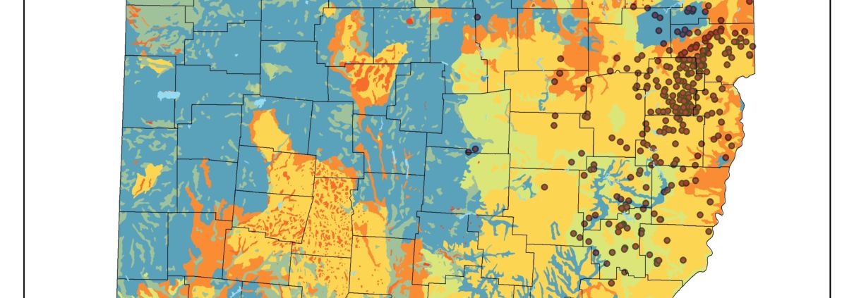
Figure 1. Ohio’s original vegetation cover and Utica Well permits as of April 30, 2013

Accordingly, the state was and is dominated by:

mixed oak (from 12,038 mi² pre-settlement to 7,911 mi² today) to the east and
maple-beech-birch (from 13,917 mi² pre-settlement to 2,521 mi² today) to the west stretching into the southeast and northwest corner of Ohio.

During pre-settlement times additional dominant forest types included:

5,181 mi² of mixed mesophytic and hemlock-beech-chestnut-red oak forests, and
3,401 square miles of oak-sugar maple (Figure 1).

Since industrialization:

The faster growing elm-ash-cottonwood has arisen as a sub-dominant forest type currently comprising 1,237 mi².
Additional sub-dominant forest types comprising 100-140 mi² of Ohio’s land area include aspen-birch (134 mi²), white-red-jack pine (124 mi²), and loblolly-shortleaf pine (108 mi²).

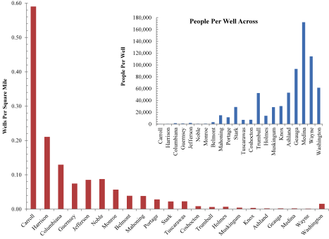
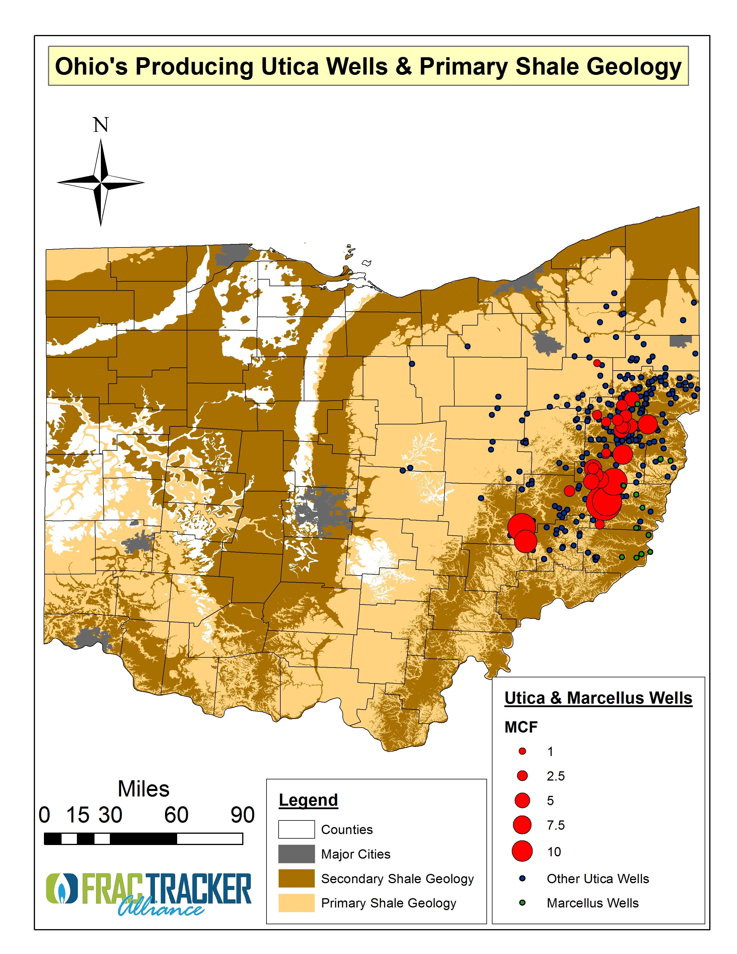
Our results suggest the average amount of deciduous forest [2] disturbed – as a percent of total well pad area – by well pad establishment is 9.8 ± 5.5% per well pad with a range of 4.7% in Stark and Holmes Counties and a high of 24% in Monroe County (Figure 2). With respect to pasture and crop displacement the average is 11.7 and 10.7% per well pad, respectively, with significantly higher between-county variability for crop cover (±5.5% Vs ±3.6%).

Figure 2. Percent Cover across Ohio’s 269 Utica Well Pads assuming an average area of 7.75 acres and the National Land Cover Database 2006 (NLCD 2006) as a proxy for previous land-use. – Click to enlarge

Converting this data into ecosystem services requires certain assumptions about plant growth, soil organic matter content, and soil compaction utilizing Natural Resource Conservation Service (NRCS) soil data to model the latter two and established peer-reviewed estimates for plant pattern and process (Follett, Kimble, & Lal, 2000; Lobell et al., 2002; Valentine et al., 2012). The basics of this analysis – assuming subsurface soils are 25% more compact and contain 45% less organic matter than the surface 12-13 inches (Needelman et al., 1999) – demonstrated that well pad establishment has displaced approximately 28,205 tons of surface and 78,348 tons of subsurface soil carbon [3] for a total of 106,554 tons of carbon equivalent to 389,986 tons of CO₂.

Additionally, the displacement and/or removal of vegetation – assuming the average Ohio forest is 40-80 years old [4] – has resulted in the annual loss of 1,050, 6,516, and 9,461 tons of crop, pasture, and forest carbon production, respectively. This is equal to 17,027 tons of carbon or 62,319 tons of CO₂, which when added to the aforementioned soil loss is equivalent to the CO₂ footprint of 25,198 Ohioans [5].

Over the life of these three ecosystem types, well pad establishment displaces 1,021,619 tons of carbon. This equates to 3.74 million tons of CO₂ or 230,034 Ohioans, which is roughly 9,000 less people than reside in Akron and Warren combined. Another way way to frame this figure is that it would be equivalent to the eightieth largest US city between Henderson, NV and Scottsdale, AZ.

At CO₂’s current valuation this Ohio Utica well pad “carbon displacement” is roughly $18.71 million. However, if we assume this is at the lower end of reasonable CO₂ estimates and that a range of $10-75 dollars is more indicative of carbon’s price, then we estimate the value of well pad displaced carbon is more like $41.29-309.68 million.

The true value of Utica well pad carbon displacement is somewhere in this range and entirely dependent on your belief in the feasibility of valuing CO₂ emissions. However, these estimates do point to some of the externalities associated with Utica Shale development currently ignored by industry lobbyists and political advocates. There is far more work to be done as it relates to understanding well pads’ influence on ecosystem services, crop productivity, and local hydrology; this is simply an attempt to begin quantifying such effects.

References

Follett, R F, Kimble, J M, & Lal, R. (2000). The Potential of U.S. Grazing Lands to Sequester Carbon and Mitigate the Greenhouse Effect. Boca Raton, FL: CRC Press LLC.

Fry, J, Xian, G, Jin, S, Dewitz, J, Homer, C, Yang, L, . . . Wickham, J. (2011). Completion of the 2006 National Land Cover Database for the Conterminous United States. PE&RS, 77(9), 858-864.

Lobell, D B, Hicke, J A, Asner, G P, Field, C B, Tucker, C J, & Los, S O. (2002). Satellite estimates of productivity and light use efficiency in United States agriculture, 1982-98. Global Change Biology, 8(8), 722-735.

Needelman, B A, Wander, M M, Bollero, G A, Boast, C W, Sims, G K, & Bullock, D G. (1999). Interaction of Tillage and Soil Texture Biologically Active Soil Organic Matter in Illinois. Soil Science Society of America Journal, 63(5), 1326-1334.

Valentine, J, Clifton-Brown, J, Hastings, A, Robson, P, Allison, G, & Smith, P. (2012). Food vs. Fuel: The use of land for lignocellulosic next generation energy crops to minimize competition with primary food production. Global Change Biology Bioenergy, 4(1), 1-19.

Footnotes

[1] The NLCD estimates land cover using sixteen classes at a 98 foot spatial resolution applied to 2006 Landsat satellite data or 4-5 years prior to the first Ohio Utica permit in September, 2010 (Fry et al., 2011)

[2] Primary tree species include red and sugar maple, red and white oak, white ash, black cherry, American beech, hickory, and tulip poplar according to the most recent USFS Forest Inventory Analysis “Ohio Forests 2006”.

[3] Along with roughly 6,536 tons of soil nitrogen assuming an Ohio soil Carbon-To-Nitrogen ratio of 14.6.

[4] Utilizing the USFS’s Forest Inventory and Analysis EVALIDator Version 1.5.1.04 tool we determined that 62% of Ohio’s oak-hickory, maple-beech-birch, elm-ash-cottonwood, and oak-pine forest types, which account for 94% of the state’s forest area, are 40-80 years old.

[5] Assuming 17.3-18.6 tons of CO2 per capita based on Oak Ridge National Laboratory’s Carbon Dioxide Information Analysis Center as cited by the World Bank.

Launch of National Mapping Project Designed to Show Possible Impacts of Oil and Gas Drilling on Well Water

May 1, 2013/by FracTracker Alliance

FOR IMMEDIATE RELEASE
US Map of Suspected Well Water Impacts
Contacts: Brook Lenker, Executive Director, FracTracker Alliance, (717) 303-0403; and
Samantha Malone, Manager of Science and Communications, FracTracker Alliance, (412) 802-0273

May 1, 2013 – The US Map of Suspected Well Water Impacts is a project that will attempt to piece together recent complaints of well water quality impacts that people believe are attributed to unconventional gas and oil operations. Research has demonstrated potential risks to ground and drinking water posed by faulty well casings, surface spills, and hydraulic fracturing. From across the country, in areas where gas and oil development is occurring, accounts of possible well water contamination have been reported but not been collected all in one place – yet. The FracTracker Alliance and cooperating organizations are providing that opportunity.

Inspired by other “crowd-sourced” data and mapping projects, this project aims to collect ongoing stories, narratives, and data from individual homeowners living on well water near drilling operations and map the general location of these reports online. The first version of the dynamic map (shown below) is available at www.fractracker.org/usmap.

US Map of Suspected Well Water Impacts - V1

US Map of Suspected Well Water Impacts
Read more about Version 1 of the map

Once received, submissions will be reviewed to the extent possible by cooperating researchers and organizations. Not all reported cases of water contamination, however, have been or will be able to be substantiated. According to Brook Lenker, Executive Director of FracTracker Alliance:

The reports we are collecting are not necessarily indisputable evidence that drilling has contaminated drinking water sources. Some accounts are irrefutable. Others remain unsubstantiated, but that doesn’t mean the well owner isn’t experiencing serious problems. Even where proof may be elusive, perception of risk can tell us much about an issue and the level of concern by the community. This information will likely help to identify pre-existing problems or conditions that were not previously well known. Such outreach is needed to permit citizens, local agencies, and others to work together to address pre-existing concerns, improve local regulations or standards, conduct proper baseline testing and monitoring, and make informed decisions.

As unconventional natural gas and oil extraction expands internationally, an Internet-based project like the US Map of Suspected Well Water Impacts can help to share on a global scale how people in the U.S. view – and may be impacted by – unconventional drilling. If everyone contributed their stories, the public’s understanding of gas and oil extraction’s impacts on well water could expand dramatically.

Anyone wishing to submit their story should visit www.fractracker.org/usmap or call (202) 639-6426. A complete list of current project partners is available on the website.

# # #

Downloadable Press Release (PDF)
Read more about Version 1 of the map

Negative Health Impacts & Stressors Perceived to Result from Marcellus Shale Activity

April 30, 2013/by Guest Author

Identified by Researchers at the University of Pittsburgh Graduate School of Public Health

By Kyle Ferrar, MPH – DrPH Candidate, Environmental and Occupational Health Department, Graduate School of Public Health, University of Pittsburgh

The potential for negative health impacts to result from unconventional natural gas development activities, such as hydraulic fracturing (deemed “frac’ing”) occurring in the Marcellus Shale basin, is a highly debated and contentious issue. To resolve this issue public health and medical professionals will need to conduct a large-scale epidemiological study – one that monitors the lives and health of a large sample of people for an extended period of time. Such a study should test to see if proximity, or closeness to unconventional natural gas development, such as frac’ing, causes negative health impacts. Such a study has not yet been officially proposed in Pennsylvania, much less funded, but researchers at the University of Pittsburgh’s Center for Healthy Environments and Communities (CHEC) believe such a study will be conducted in the future.

New peer-reviewed research released by the CHEC provides background data for that kind of study. The research documented 59 unique health impacts, or “symptoms,” and 13 “stressors” perceived to result from Marcellus Shale development. Over time, symptoms and perceived health impacts increased for the sample population (p<0.05), while stressors resulting from Marcellus Shale activity remained consistent (p=0.60). The study group was a biased sample population, meaning the participants were not randomly selected. Rather, the participants were already concerned by or interested in issues associated with this industrial activity.

Using community based participatory research methods, researchers from CHEC, along with researchers from FracTracker while it was still a project at CHEC, engaged community members with in-depth interviews. Mail surveys have been conducted by other researchers in Colorado and Wyoming, but this is the first research to use an ethnographical, in-person approach. Furthermore, this is the first peer-reviewed and published research that describes symptoms in those who believe their health has been affected. The six most reported symptoms are reported in Table 1, with stress being the most commonly reported health effect.

The article contributes several new findings to this field of research, including evidence about what people report as stressors. Contributions of stress to negative health effects are well documented in the literature, known as allostatic loads. The six most commonly reported “stressors,” or sources of stress, are reported in Table 2. Particularly notable is the very high percentage of the group that report issues such as being lied to that presumably would be corrected if the industry became more transparent and responsive. The article also reports on the longitudinal nature of the perceived health impacts and stressors. Longitudinal refers to the fact that the data were collected over time, not just once. Follow-up interviews conducted 19-22 months after the initial interviews showed that the number of perceived health impacts reported by participants actually increased over time, while the number of stressors reported remained consistent. This contradicts industry’s argument that the problems are mainly caused by seeing and hearing drilling activity, and that as the intensity of activity diminishes over time so will the symptoms and stressors. While this research does not answer the larger question of whether negative health effects are associated with Marcellus Shale development, it demonstrates a need for future studies to be conducted within these particular communities and supports the more difficult task of embarking on a broader epidemiological study.

Table 1. Most reported symptoms with the percentage of participants reporting said symptom.

Symptoms	Session 1 (n=33)
Stress	76%
Rashes	27%
Loss of sleep	27%
General illness	24%
Headaches	24%
Diarrhea	24%
Shortness of breath	21%

Table 2. Most reported “stressors” participants associated with Marcellus Shale development, with the percentage of participants reporting said stressor.

Stressor	Session 1 (n=33)
Denied or provided false information	79%
Corruption	61%
Concerns/complaints ignored	58%
Being taken advantage of	52%
Financial damages	45%
Noise pollution	45%

About the Journal Article

Assessment and longitudinal analysis of health impacts and stressors perceived to result from unconventional shale gas development in the Marcellus Shale region <-- Note: This link is presently not connecting to the article on IngentaConnect.com. We will update the link once the article becomes available again on their site. Authors: Kyle J. Ferrar; Jill Kriesky; Charles L. Christen; Lynne P. Marshall; Samantha L. Malone; Ravi K. Sharma; Drew R. Michanowicz; Bernard D. Goldstein Source: International Journal of Occupational and Environmental Health

A Year in the Life of Ohio’s Utica Play

April 23, 2013/by Ted Auch, PhD

The Ohio Utica play has taken off in the last calendar year, jumping from 160 permitted wells as of March 2012 to 453 since then. This equates to 1.24 permitted wells per day. (Note: The state’s less exploited Marcellus shale had 13 permitted wells a year ago with an increase of 7 since then.) A year ago Ohio was home to 50 “drilled” wells and is now home to an additional 80 “drilled” wells (Figure 1). Meanwhile 0.65% and 1.14% of permitted wells are what Ohio Department of Natural Resources (ODNR) calls “Inactive” or “Not Drilled” with the latter being relatively similar a year ago vs. today with 3 and 4 “Not Drilled” wells, respectively. According to the latest ODNR data 54 Utica wells were permitted as of 4/1/2012 vs. 342 since then. Plugged wells constitute 1.63% of all Ohio Utica wells although the industry appears to be increasing efficiency with respect to plugging having experienced 7 “Plugged” wells as of 4/1/2012 and only 3 since. Conversely, wells that are “Producing” have declined from 25.63% (41 “Producing” wells) of all permitted wells to 1.32% (6 “Producing” wells) of all permitted wells since then with the latest reported producing well being a Mountaineer Keystone well in Windham Township, Portage County.

The permitting process has continued along its exponential path since permitting began September 28, 2010 (Figure 2). The gross average number of permitted Ohio Utica wells per month in the last five months is 39 with a total of 195 permitted since November 2012. The quarterly permit average has increased by an order of magnitude of 4.2 permits per month between September 2010 and 2011 to 39 per month since September 2012. In recent months Washington county was added to the list of Ohio counties home to Utica hydraulic fracturing permits, while Carroll remains the state with the most Utica permits followed by Harrison, Columbiana, Guernsey, and Jefferson/Noble with the average number of Utica well permits across the 22 counties home to at least one permit being 28 per county with six counties above and sixteen below this mean (Figure 3). In the last year the four counties that have entered the Utica conversation are Trumbull, neighboring Holmes and Wayne, and Washington, with 4, 3, 1, and 1 Utica permit as of April 1^st, respectively. Meanwhile five other counties have seen no increase in Utica permits including Muskingum, Knox, Ashland, Geauga, and Medina. Conversely Belmont County has seen a 21-fold increase in Utica well permits followed distantly by Harrison, Guernsey, Noble, and Coshocton counties all of which have experienced ≥5-fold increases.

The average number of people per Utica well across the aforementioned 22 counties is 31,808, while the average number of wells per square mile is 0.066. The range is quite broad for both variables ranging from 0.0018 wells per square mile in Wayne – home to the Wayne National Forest – to 0.59 wells per square mile in Carroll County, with the one recent Washington County well placing it 13^th out of 22 counties. The inverse is the case for people per well with Medina County, home to the highest number of people relative to Utica well permits with 172,332 people per well (vs. 124-563 people per well in Carroll, Harrison, Noble, and Monroe counties). Since last we conducted this type of analysis in late January the valuation of Ohio’s major Utica players has actually increased by 11.7%. This is a particularly complex situation considering that Atlas Noble the owner of 6 Utica wells has actually gone private for a variety of reasons and Chesapeake Energy has ousted its CEO Aubrey McClendon due to “philosophical differences and a pending SEC investigation. Meanwhile, Wall Street-types:

… expect well results to vary greatly, given 2012 drilling activity across many fringe areas of the play. We believe weak results from other operators are likely to validate that Gulfport remains the most exposed operator. Source

Additionally, the repeated delay in 2012 production numbers scheduled for the 1^st of April is creating layer upon layer of uncertainty leaving everyone guessing and relying on 2011 production numbers. This leaves public sentiment worried about the unsustainability, uncoordinated, and unbalanced nature of both Ohio’s regulatory framework and highly Utica exposed and/or leveraged balance sheets. Meanwhile Wall Street analysts are contemplating whether market forces, expectations, reality, or collusion is to blame. Our current model of potential Utica production in the form of barrels of oil equivalent speaks to small and discrete highly productive zones in Belmont, Noble, Guernsey, Morgan, and Muskingum counties, rather than the originally estimated zones of highest production in Carroll and Columbiana. An additional hotspot appears to be located in Fairfield, Perry, and Hocking counties. However, due to insufficient data quantity, quality, and methodology, and transparency from ODNR and industry, the opportunities to conduct such exercises are still accompanied by substantial uncertainty in the form of high signal-to-noise resulting from scant and unreliable data. The hope, herein and on Wall Street, is that ODNR and industry will begin to make their production data available in real-time.

This is an especially important consideration given that the aforementioned regulatory environment here in Ohio – as well as the relatively generous severance taxing system [1] – has reached a point that even industry/supply-side think tanks like The Fraser Institute in Canada have determined “the extent of investment barriers (based on All-Inclusive Composite Index values)” are as good as they are ever going to get; Ohio trails only Mississippi in a global investment barrier ranking of 146 countries, US states, and Canadian provinces. Furthermore, in one year the conditions for doing largely hydrocarbon-related business in Ohio improved so much between 2010 and 2011 that Ohio jumped up the league tables from 12^th to 2^nd, according to the institute’s 2011 “Global Petroleum Survey.” This loosening of regulations, combined with decreasing data quality and availability, is the primary concern of The FracTracker Alliance in Ohio.

Figure 1: Utica Permit activity by status to April 1, 2013

Figure 2. Cumulative and Per Month Utica Permits to September 2010 through March 2013

Figure 3. Utica Permit Count by County from September 28, 2010 to April 1, 2013

Figure 4. Utica Permits Per Square Mile and People Per Well by County from September 28, 2010 to April 1, 2013

(Note: This model was constructing utilizing the Geostatistical Analyst Tools “Empirical Bayesian Kriging” tool in ArcGIS)

Figure 5. A map of the current Ohio Shale and Tight Gas Plays, hydraulic fracturing permits in Ohio as of 4/1/2013, and a generalized model of potential production from with light green representing 20 Barrels of Oil Equivalent (BOE) and red approximately 10,000 BOE

Table 1. Distribution of Ohio Utica Shale wells across companies (#, %), Date of First Permit (DFP), and the valuation of the publicly funded companies at their DFP at the close of business 4/9/2013.

				Company Valuation
Company	#	%	DFP^†	Share Price DFP	Share Price 4/9/2013	% Change
Anadarko^•	12	0.019	09/07/2011	69.88	86.70	1.241
Antero	21	0.034	03/23/2012
Atlas Noble^††	6	0.010	09/24/2012	31.14
Carrizo	2	0.003	07/26/2012	24.02	26.26	1.093
Chesapeake Energy^•	389	0.626	12/23/2010	25.61	19.99	0.781
Chevron Appalachia	2	0.003	07/31/2012	109.58	118.71	1.083
Consol Energy^•	25	0.040	06/17/2011	45.86	33.85	0.738
Devon Energy	13	0.021	11/02/2011	65.46	55.28	0.844
Eclipse Resources	1	0.002	12/21/2012	—	—
Enervest^•	16	0.026	06/30/2011	9.37	8.79	0.938
EQT	3	0.005	09/13/2012	57.76	69.59	1.205
Gulfport Energy^•	46	0.074	02/28/2012	35.49	48.09	1.355
Halcon	2	0.003	11/02/2012	5.003	7.69	1.537
Hall Drilling	1	0.002	09/17/2012
Hess Ohio	24	0.039	09/28/2010	53.63	73.50	1.371
HG Energy	16	0.026	09/14/2011	—	—	—
Hilcorp Energy	3	0.005	12/14/2012	—	—	—
Mountaineer Keystone	7	0.011	07/13/2012	—	—	—
PDC Energy^•	9	0.014	05/25/2012	25.67	47.59	1.854
R E Gas Development^•	13	0.021	03/19/2012	—	—	—
Sierra Resources	3	0.005	07/02/2012	—	—	—
SWEPI	1	0.002	06/20/2012	—	—	—
XTO Energy	5	0.008	04/09/2012	0.28	0.01	0.036
BP	1	0.002	03/20/2013
	613					1.083

^† DFP = Date of First Permit; “—“ not a publicly traded company

^†† Atlas Noble has since gone private

^• Corporations that have reported production numbers as of this post: 1) Anadarko – 3, 2) Chesapeake – 14, 3) Consol Energy – 1, 4) Enervest and PDC Energy – 2, 5) Gulfport – 10, R E Gas Development – 4.

[1] Ernst & Young in a 2011 report found that Ohio’s hydrocarbon taxing rates were the most favorable of the eight states they investigated with a total state and local tax of 1.8% vs. 10.9-11.0% in neighboring West Virginia and Oklahoma, respectively. The average across the seven other states was 9.2% or 5.12 times that of The Buckeye State.

US Pipelines Incidents Are a Daily Occurrence

April 15, 2013/by Matt Kelso, BA

Recently, there has been a lot of attention focused on the Mayflower, Arkansas pipeline failure that resulted in a massive oil spill, particularly as it comes at a time when discussions of the controversial Keystone XL Pipeline project are once again heating up. However, the situation is far from unusual. In fact, according to data downloaded from the Pipeline and Hazardous Materials Safety Administration (PHMSA), there were 1,887 incidents in the nation’s gathering and transmission, distribution, and hazardous liquids pipelines between January 1, 2010 and March 29, 2013, or an average of 1.6 incidents per day.

Pipeline incidents from 1/1/2010 through 3/29/2013. Data Source: PHMSA.

Obviously, not all of these failures are on par with the massive spill in Mayflower, and it should be noted that there are a variety of reasons for these lines to fail. Some of these reasons, such as excavation activity in the vicinity of a pipeline, are not necessarily the fault of the pipeline’s operator. The fact that these incidents are commonplace, however, is not one that can be dismissed.

Pipeline incidents in the United States from 1/1/2010 through 3/29/2013. Source: PHMSA. Red Triangles represent incidents leading to fatalities, and yellow triangles represent those leading to injuries. To access the legend and other controls, click the “Fullscreen” icon at the top-right corner of the map.

It is clear from the map that there a few data entry errors, as a few of the data points draw in locations that aren’t even in the jurisdiction of the United States. However, each entry also contains a city and state that the incident is associated with, and for the most part, the data seem to be fairly reliable.

PACWA’s List of the Harmed Now Mapped by FracTracker

March 7, 2013/by Matt Kelso, BA

Jenny Lisak, co-director of the Pennsylvania Alliance for Clean Water and Air, maintains a list of people claiming to be harmed by hydraulic fracturing or related processes, called the List of the Harmed. This version of the list, last updated on February 23, 2013, has 822 people thought to be negatively impacted by the industry, with symptoms ranging from headaches and rashes to death.

The List of the Harmed is maintained by the Pennsylvania Alliance for Clean Water and Air. For full access to map controls, click the “Fullscreen” icon at the top right corner of the map.

The FracTracker Alliance was not involved in the creation or maintenance of this list, but our intern Stephen Paddock did map the incidents to the best available level of accuracy, whether that was at the municipal, county, or state level. Please do not assume that the locations on the map are any more accurate than the level indicated in the “Accuracy” column.

Popup box containing the data for one of the 878 entries on the List. The yellow oval shows that there are multiple boxes stacked on top of each other, and the green oval provides a hyperlink to more information about the incident in question.

Each entry on the List of the Harmed has at least one link to more information about the given incident. To access those, click on any map icon to bring up the popup box. Then scroll down to the “Link” section, and click on “More info”. If there are multiple sources, they will appear under “Link_2” or “Link_3”.

In the picture above, the text “(1 of 11)” in the yellow oval tells us that there are eleven popup boxes stacked on top on one another. To sort through the records, simply click the arrow button toward the right edge of the yellow oval.

Waste produced by unconventional wells in Pennsylvania from June to December 2012.

Six Months of Production and Waste From PA’s Unconventional Wells

March 1, 2013/by Matt Kelso, BA

The Pennsylvania Department of Environmental Protection (DEP) recently published its biannual reports for production and waste from unconventional wells throughout the state for the last half of 2012. FracTracker has learned the hard way not to be too eager in analyzing this data. In the previous cycle, this data was released without the contribution several operators, one of which happened to be the biggest player in the state, Chesapeake Appalachia. That incident prompted the inclusion of a data disclaimer from DEP, which includes the following text:

The Oil and Gas Act reporting is a self-reporting system, meaning that data is reported from producers to DEP as required by law. All production data is posted as it was received from the unconventional well operators. DEP does not independently verify the data before it is posted.

While the Oil and Gas Act requires accurate and on-time data reporting by producers, and the producers and DEP endeavor to correct any errors discovered after the data is posted, DEP makes no claims, promises or guarantees regarding the accuracy, completeness or timeliness of the operators’ data that DEP is required to post.

While considering content regarding production and waste in Pennsylvania, it is worth noting that the DEP considers the data to belong to the various operators. All data for this post was downloaded on February 25, 2013, and while it seems reasonably complete, it is important to note that there could be operators which have not posted their data to DEP in a timely fashion.

PA Production and Waste From Unconventional Wells: July 2012 to December 2012. Click on any map icon for more information, or click the “Fullscreen” button at the top right of the map to access more toolbars. To access data for individual wells, viewers must zoom in to 1:750,000, or an area equivalent to several counties.

The default map frame includes most of the activity for unconventional oil and gas production and waste from Pennsylvania, but if you zoom out, you can find a landfill in southwestern Idaho that accepted 11 tons of flowback fracturing sand for disposal. Unfortunately, the available data does not give any indication of why an operator might choose to ship waste over 2,000 miles away from its source.

Below are the six month statewide production and waste totals for Pennsylvania’s unconventional wells, including the number of wells that contributed to each total:

Production from unconventional wells in Pennsylvania from July to December 2012. Mcf represents 1,000 cubic feet, and barrels measure 42 US gallons.

The total gas produced was over 1.1 trillion cubic feet (Tcf) for the six month period, which was over 250 billion cubic feet (Bcf) higher than the previous total of 895 Bcf.

Waste produced by unconventional wells in Pennsylvania from June to December 2012.

And here is a look at the disposal method for each type of waste, in terms of percentage:

Disposal methods of Pennsylvania unconventional oil and gas waste products, in terms of percentage of the waste type. July – December 2012.

Note that while road spreading rounds down to 0%, 425 barrels of produced fluid were used in this effort.

To Severance Tax or not to Severance Tax, that is the question!

February 25, 2013/by Ted Auch, PhD

By Ted Auch, PhD – OH Program Coordinator, FracTracker Alliance

Million Cubic Feet (MCF) as measured over industry standard test periods.

Figure 1. Ohio’s Producing Utica Wells & Primary Shale Geology – plus non-reporting, drilled, or producing Utica & Marcellus Wells.
“Million Cubic Feet” (MCF) as measured over industry standard test periods.
“Barrels of Oil Equivalents” (BOE) as measured over industry standard test periods.

The economic opportunities provided by Ohio’s Utica Shale play via hydraulic fracturing have been cited repeatedly by the Ohio Oil and Gas Association and industry think-tanks like IHS Inc [1]. Numbers published by the latter last October [2] predicted 143,000 Ohio jobs and $18 billion in state revenue by 2020. However, these projections are accompanied by substantial amounts of error. Given that the state’s Utica Shale well movement is now more than 500 wells permitted strong, we thought it was time to take a closer look at the demographics and economics of the Utica Play, given that there will be a strong geographic component being inserted into the “To Drill Or Not To Drill” and waste disposal debate here in Ohio. This is an especially important issue given that the state is wrestling with either implementing an ad valorem [3] tax or raising the state’s industry-low severance taxes, which currently stands at 0.5-0.8% but would be raised to 1% under the governor’s budget. In contrast, proposals from Policy Matters Ohio and northeast Ohio Democrats seek 5% – 7%, respectively.

In comparison to most other states producing oil and gas, even 5% may be a trivial amount, or what The Cleveland Plain Dealer called “indefensibly low.” It amounts to 97 cents per Ohioan (i.e., $275 mi²) [4]. According to an Ernst & Young analysis of eight states that produce dry gas and natural gas liquids and/or dry gas and oil…

Ohio currently imposes the lowest combined state and local taxes of the states included in the analysis.
…Ohio’s overall effective tax rate (measured as total taxes divided by sales) is 80% below the average rate for the other 7 states for a well producing dry natural gas and natural gas liquids.
For a well producing dry natural gas and oil, Ohio’s effective tax rate is 65% below the other-state average…
With the [proposed] increase, Ohio’s effective severance tax rate (ETR) would be 16% lower than the other states’ average for the well producing dry natural gas liquids and 4% lower than the other states’ average for the well producing dry natural gas and oil.

The governor’s proposed “Severance Tax Changes” will not apply to any Marcellus Shale wells, even though the state is home to five producing Marcellus wells (two in Monroe County) and eight permitted wells across Belmont and Monroe Counties. Additionally, the governor and his staff included a severance tax exemption for all “small-volume gas wells” (gas wells with average daily production of under 10 million cubic feet [MCF] would be exempt from the tax). If early industry production reports – and the Ohio Business Roundtable requested Ernst & Young report – are any indication, only 19% of wells will be subject to this tax. Our own analysis revealed that of the 32 industry reported production wells, the average production value is 7.5 MCF (Figure 1).The Kasich administration admitted the exemptions would apply to – by their estimation – 45,000 gas wells.

Another nuance of the Kasich administration’s severance tax complicated mélange is that rates will be 1% for natural gas and 4% for oil, natural gas liquids, and condensate. However, according to the administration:

… there will be a lower tax rate of 1.5 percent for the first year of production, in order to allow producers to recover the cost of preparing the well site and drilling the well.

Coincidentally, “the first year of production” is generally the time of greatest gas yields. Anonymous sources in Ohio’s Utica sweet spot have spoken of 50% declines in royalties within 6 months of production.

The Ohio Oil and Gas Association, the industry’s lobbying arm, has weighed-in against higher severance taxes, stating that:

a 4% severance tax on oil and gas would be equivalent to a 40% income tax and 16 times more than the commercial activities tax (or CAT). It would also burden economically challenged area throughout the state and landowners who want to lease their land and receive royalty streams.

(Total of 4,037 individual donations, Data courtesy of Common Cause Ohio’s “Deep Drilling, Deep Pockets: Campaign Cash and Fracking Regulation in Ohio” spreadsheet)

Figure 2. Ohio’s Big Energy individual or Political Action Committee (PAC) political donations from 2001 to 2011. (Total: 4,037 individual donations. Data courtesy of Common Cause Ohio’s Deep Drilling, Deep Pockets spreadsheet.)

The anonymous BizzyBlog took the OOGA position one step further proclaiming that energy companies “won’t do business in a state with a newly-enacted punitive severance tax.”

Such arguments against a “hefty tax increase” don’t have much empirical support. OSU oil and gas development expert Douglas Southgate called such taxes “definitely affordable for the industry.” Even with the increases proposed by some, Ohio would still rank lowest among the eight shale gas producing states investigated by Ernst & Young in 2012.

Whereas an ad valorem tax would be redistributed directly back into the communities from which the hydrocarbons are extracted, a severance tax would be distributed throughout the state, even to communities and counties that prohibit Utica Shale drilling and/or injection activity. Theoretically, the entire state could benefit from the toils and environmental risks taken on by Ohio’s Appalachian region. According to a Quinnipiac pole, Ohioans support (52 to 38%) an increase in drilling-related severance taxes. Bipartisan voter support for a severance tax increases (60 to 32%) when the prospect of offsetting state income taxes is proposed.

Either levy – an ad valorem tax or severance tax – would be based upon the industry’s headline well production, even though USGS research recently spoke to the substantial well-to-well production variability in the Appalachian Shale Basin: 250-600% [5]. There are quite a few short- and long-term costs and benefits associated with exploitation of the Utica Shale; however, as it stands the risk burden is disproportionately being shouldered by Appalachian Ohio. Thus, the severance tax being proposed by the governor and House Democrats could add to the regional schisms evident in the state.

But maybe geography is immaterial. The likely big winner of the tax decisions will be energy companies and, according to data on recent campaign contributions, those politicians they deem worthy of their political donations – many of whom are on the fringes or completely outside the Utica Shale (Figure 2).

[1] IHS Global Insight is the brainchild of Daniel Yergin.

[2] This work was funded by the US Chamber of Commerce’s Institute for 21^st Century Energy, the American Petroleum Institute, the American Chemistry Council, America’s natural Gas Alliance, and the Natural Gas Supply Association.

[3] Ad valorem taxes are assessed according to the value of the natural gas extracted.

[4] The Kasich “Ohio’s Jobs Budget 2.0: Jobs. Momentum. Transformation” highlights this aspect of their proposed severance tax, explicitly noting that it “has researched the severance tax structures of other states with significant oil and gas production, particularly those states with shale resources, and has found that even with a 4 percent tax rate, the tax burden on the revenues from these horizontal Utica wells will be lower than in other states.”

[5] According to the USGS, production from the most productive wells in the Appalachian Basin’s shale formations is commonly 50 times larger than the poorest producing wells, with the same value being 250-600 times larger for the Marcellus Basin. However, the only numbers presented to individual landowners – but less frequently to collectives given that energy firms are increasingly aware of the legal advice that land aggregators are seeking out – when the subject of royalties comes up are near-term gushers. For example:

GPOR’s “’King’ of Utica Well” the Shugert 1-1H at 4,913 barrels of oil equivalents per day (BOEPD),
CHK’s Buell well in Harrison County, OH producing 1,040 BOE[5],
GPOR’s Boy Scout 1-33H in Wagner, Harrison County producing 3,456 BOE, the Ryser 1-25H producing 2,914, or the Groh 1-12H producing 1,935 BOE,
Anadarko’s 9,5000 BOE, and
The Wagner 1-H well producing 4,650 BOE. Yet, wells like the Frank unit in Stark County owned by Enervest producing 515 BOE or the non-producing wells across Ashland and Medina Counties are barely discussed – what a JP Morgan energy analyst called a “funding gap.”

New Michigan Map Shows off New FracMapper Functionality

February 21, 2013/by Matt Kelso, BA

This page was updated in January 2018 to fix the embed code in the map.

Recently, FracTracker has been getting requests from residents in many locations to map large-scale oil and gas operations in their area. We now have content for Michigan, which happens to correspond with the release of additional map export functionality on FracMapper:

View map fullscreen | How FracTracker maps work

About the Michigan Data

Each state is different in the data it makes available to the public, so it is always interesting to take a look at how new areas approach their duties of data transparency. After having recently produced maps for New Mexico and Colorado, I confess to being excited to work with data from a state that embraces designating locations in latitude and longitude (and doesn’t release data only with the archaic PLSS notation). But then, sometimes mapmakers are easy to please.

Far more important is the data made available for wells related to oil and gas development by the Michigan Department of Environmental Quality. Not only does it include the standard well type designations of “oil” or “gas”, but it also includes observation wells, storage wells, and injection wells. Altogether, there are 15 categories of well types.

As with many states, there are so many legacy oil and gas wells that mapping them all would overwhelm the online mapping software servers with data requests from over 63,000 wells. For that reason, the wells are restricted to those marked as being horizontally drilled, which reduces that number to 1,562. That should include most of the unconventional oil and gas extraction activity from recent years.

Also included in the data are point locations for the tops and bottoms of the well bore, which could be used in the future to map a generalized path of the horizontal wells beneath the surface.

FracMapper Export Feature Enhancement

The Michigan map is the first one produced with our new “Save as PDF” tool, which can be found in the “Export” toolbar.

The “Save as PDF” tool in the the Export Menu creates as landscape oriented 8.5″ x 11″ document, complete with title, scale bar, and legend. The legend contains only those map icons that are displayed in the view of the PDF.

Please note that if you wish to make multiple PDF files from the same map, it is currently required to refresh the webpage containing the map, or it will continue to produce the same map.

In the coming weeks, this functionality will be added to the other FracMapper entries that have already been published. We are also hoping to roll out additional functionality in the near future.

Learn More

About Oil and Gas Activity in Michigan

NM Shale Map Shows Contamination Events

January 30, 2013/by Matt Kelso, BA

Recently, the FracTracker Alliance has gotten several requests from residents of New Mexico for maps showing the large scale drilling operations in that state. As we began to look around for data sources, we encountered an interesting document from 2008:

This 2008 document from the New Mexico Oil Conservation Division shows instances of ground water contamination by oil and gas pits in the state.

There isn’t much description on the document or the New Mexcio Oil Conservation Division (NMOCD) page that links to it, however, the subject matter is straightforward enough. Altogether, there are 369 instances of ground water contamination documented by a New Mexico governmental agency from dozens of drilling operators throughout the Land of Enchantment.

Ground Water Contamination Controversy

Since the title of document indicates that the agents causing contamination are “pit substances”, this does not technically indicate that hydraulic fracturing is to blame. This is largely a matter of definition, but it is an important one to understand, because the word “fracking” means something different to industry insiders than it does to the general public, and the issue of ground water contamination is a point of considerable debate.

Technically speaking, hydraulic fracturing only refers to one stage of the well completion process, in which water, sand, and chemicals are injected into the oil or gas well, and pressurized to break up the carbon-rich rock formation to allow the desired product to flow better.Most people (and many media outlets) consider “fracking” to be the entire production process for wells that require such treatment, from the development of the several acre well pad, through the drilling, the completion, flaring, waste disposal, and integration of the product to pipelines. (It is due to these competing definitions that the FracTracker Alliance goes out of our way to avoid the term “fracking”.)

All of this has lead to some carefully worded statements that seem to exhonerate hydraulic fracturing, despite suspected contamination events reported in Pennsylvania, Wyoming, and elsewhere. Of course, from the perspective of residents relying on a contaminated aquifer, it hardly matters whether the water was contaminated by hydraulic fracturing, leeching from the associated pits, problems with well casing or cement, or re-pressurized abandoned wells. A fouled aquifer is a fouled aquifer.

This document does not specify what was contained in the pits, only that they are contamination events. Therefore, we do not know what stage of the process the contaminant came from, only that it was believed by the state of New Mexico to have originated from a pit, and not the well bore itself.

Notes About Location Information

It is important to note that the location information is not exact, but are generally within 0.72 miles of the specified location. The reason for this is that the location information was provided using the Public Land Survey System (PLSS). The brainchild of Thomas Jefferson, the PLSS was the method used to grid out the western frontier, and it is still used as a legal land description in many western states. Essentially, the land was divided into townships that were six miles by six miles, which was then broken into 36 sections, each of which is one square mile. FracTracker has calculated the centroid of each section, which could be up to 0.71 miles from the corner of the same section if the shape is perfectly square.

The PLSS system was used to grid out most of New Mexico, but some portions of the state had already been well defined by Spanish and Mexcian land grants. Aside from being a fascinating historical anecdote, it does have an effect on the mapping of these pits. In the image of the table above, note that the “Florance Z 40” well does not have any values in the location column. As a result, we were not able to map this pit. Altogether, 11 of the 369 pits identified as causing groundwater contamination could not be mapped.

New Mexico Shale Viewer. You can zoom and click on map icons in this window for more information. For full access to map controls, including layer descriptions, please click the expanding arrows icon in the top right portion of the map.