By Ted Auch, OH Program Coordinator, FracTracker Alliance
Ohio is the only shale gas state in the Marcellus and/or Utica Shale Basin that has decided to go “all in.” i.e. The state is moving forward with shale gas production, Class II Injection Well disposal of brine waste from fracking, and more recently the processing and disposal of drill cuttings/muds via the state’s Solid Waste Disposal (SWD) districts and waste landfills. The latter would fall under the joint ODNR, ODH, and EPA’s September 18, 2012 Solidification and Disposal Activities Associated with Drilling-Related Wastes advisory. It occurred to us that it might be time to try to estimate how much of these materials are produced here in Ohio on a per-well basis using basic math, data gleaned from Ohio’s current inventory of Utica wells and the current inventory of PLAT maps, and some broad assumptions as to the density of Ohio’s geology.
Developing the Estimate
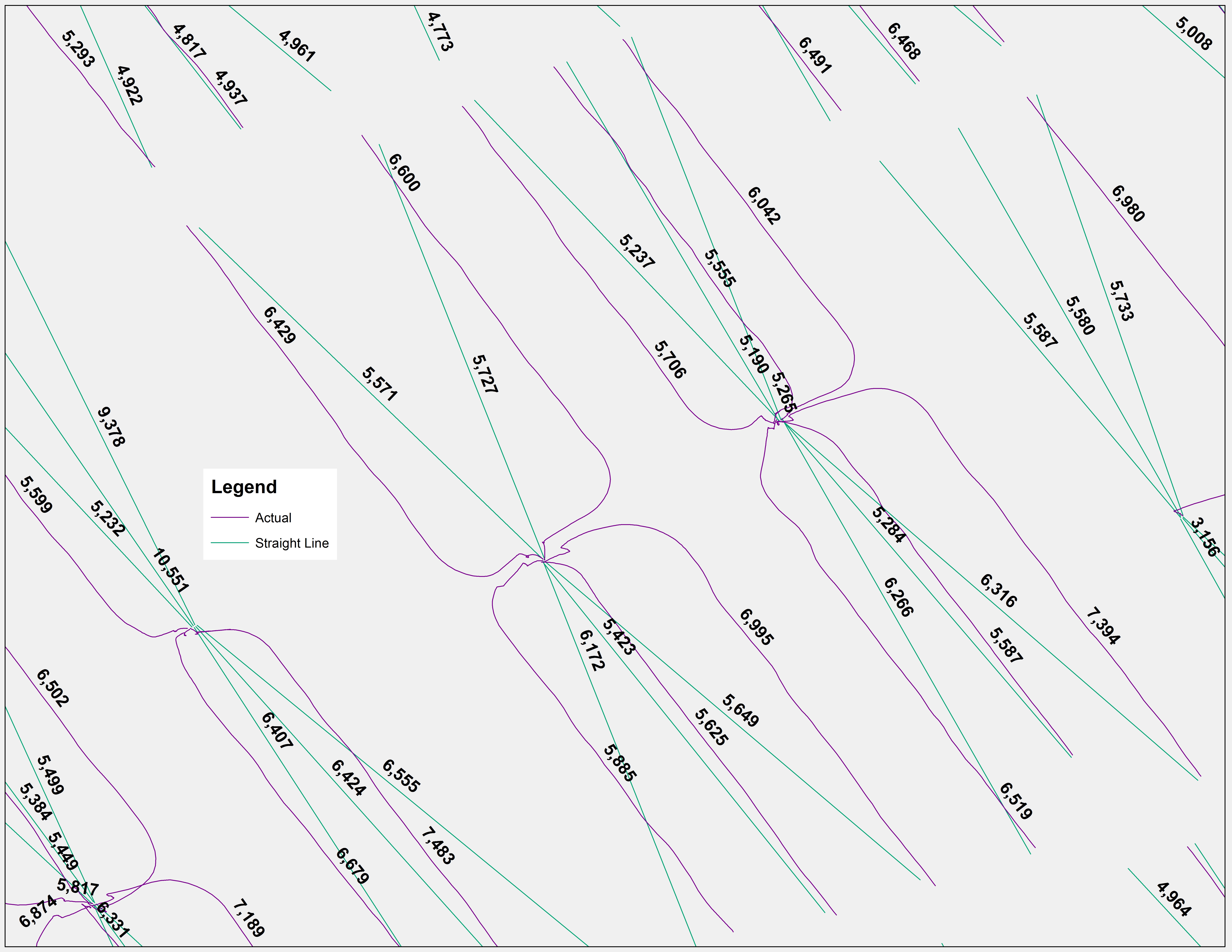
1) Start with a 341 Actual Utica well lateral dataset generated utilizing the ODNR Ohio Oil & Gas Well Database PLAT inventory or the current inventory of 1,137 permitted Utica wells. Generate a Straight Line lateral dataset by converting this data from “XY To Line” with the following summary statistics:
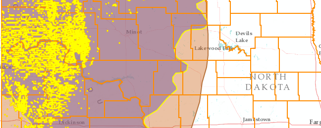
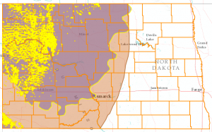
Average Lateral + Vertical Footage = 13,205-13,261 total feet (402,488-404,195 centimeters) (Figure 1)
Fig. 1. An example of Actual and Straight Line Utica well laterals in Southeast Carroll County, Ohio
3) We assume a rough diameter of 8″ down to 5″ (20-13 centimeters) for all of 1) and 14″ to 8″ (36-20 centimeters) for the entirety of 2)
4) The density of 1) is roughly 2.61 g cm3 assuming the average of seven regional shale formations (Manger, 1963)
5) None of the materials being drilled through are igneous or metamorphic (limestone, siltstone, sandstone, and coal) thus the density of 2) is all going to be
≈2.75 g cm3
6) The volume of the above is calculated assuming the volume of a cylinder
(i.e., V = hπr2):
Σ of Actual Lateral Length 49,205,721 cm3 * 2.61 g = 128,180,904 g
Σ of Actual Lateral Length 153,991,464 cm3 * 2.75 g = 423,476,526 g
Average Lateral + Vertical Volume = 551,657,430 grams = 1,216,195 pounds =
608 tons of drill cuttings per Utica well * 829 drilled, drilling, or producing wells = 504,113 million tons
The coarse assumptions as to density of materials and the fact that these materials experience significant increases in surface area once they have been drilled through.
The assumptions as to pipe diameter could be over or underestimating drill cuttings due to the fact that we know laterals taper as they near their endpoint. We assume 45% of the vertical depth is comprised of 14″ diameter pipe, 40% 11″ diameter pipe, and 15% 8″ pipe. Similarly we assume the same percentage distribution for 8″, 6.5″, and 5″ lateral pipe.
Ohio Drilling Mud Generation and Processing
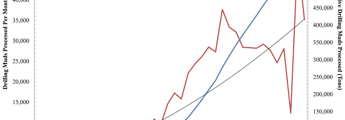
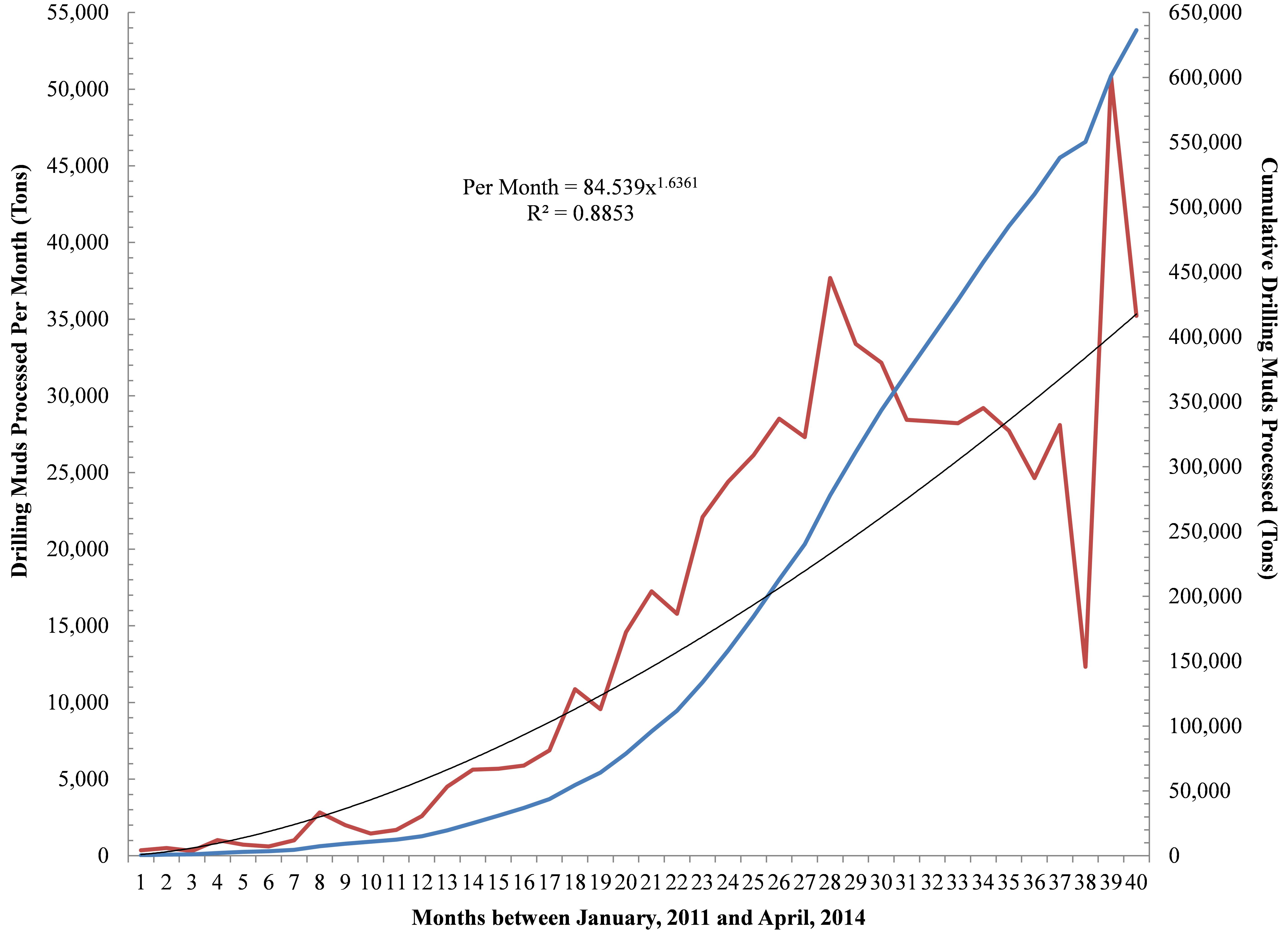
Fig. 2. Month-to-month and cumulative drilling muds processed by CCHSWD, one of six OH SWDs charged with processing shale gas drilling waste from OH, WV, and PA.
Ohio’s primary SWDs responsible for handling the above waste streams – from in state as well as from Pennsylvania and West Virginia – are the six southeastern SWDs along with the counties of Portage and Mahoning according to several anonymous sources. However, when attempting to acquire numbers that speak to the flows/stocks of fracking related SWD waste (i.e., drilling muds) the only district that keeps track of this data is the Carroll-Columbiana-Harrison Solid Waste District (CCHSWD). The CCHSWD’s Director of Administration was generous enough to provide us with this data. According to a month-over-month analysis they have processed 636,450 tons generating a fixed fee of $3.5 per ton or $2.23 million to date (Figure 2). This trend translates into a 1,046-1,571 ton monthly increase depending on how you fit your trend line to the data (i.e., linear Vs power functions) or put another way annual drilling mud increases of 12,546-18,847 tons.
https://www.fractracker.org/a5ej20sjfwe/wp-content/uploads/2014/05/SWD_DrillingMuds-scaled.jpg10891500Ted Auch, PhDhttps://www.fractracker.org/a5ej20sjfwe/wp-content/uploads/2025/09/2025-Wordmark-Logo.pngTed Auch, PhD2014-05-08 13:36:222020-07-21 10:42:26Utica Shale Drill Cuttings Production – Back of the Envelope Recipe
By Ted Auch, OH Program Coordinator, FracTracker Alliance
The “Why?”
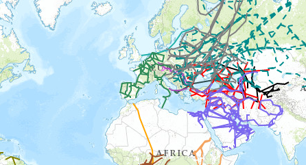
Recently, the US has proposed to ship American shale gas abroad to buffer Europe’s 15-30% reliance on Russian gas imports in the face of the annexation of Crimea by Russia – and parallel 80% increases in LNG prices paid by Eastern Europeans to Russia’s Gazprom. The FracTracker map below illustrates all proposed and existing hydrocarbon pipelines across South America, Africa, Europe, the Persian Gulf, and Asia/Russia1. Creating such a map seems the least we could do given that this conflict has been called the “worst crisis with the West since the end of the Cold War.” The situation in Crimea is a chronic crisis; folks like Oxford University’s Jonathan Stern have suggested:
Ukraine owes Gazprom $2 billion for already delivered hydrocarbons,
Russia can easily turn their supplies to Japan which will pay a premium relative to what they are getting from the European Union, and
The duration of European oil and gas contracts with Gazprom, which extend 15-35 years, can’t be broken (Einhorn, 2014; Henderson and Stern, 2014).
The rhetoric framing here in the US has been lead by – and regurgitated by media outlets such as NPR who suggested “Putin Could Send Europe Scrambling For Energy Sources” – the likes of the Council on Foreign Relations Richard Haass and the Brookings Institution’s Bruce Jones. Both of these entities have the ears of congress domestically and global decision makers at gatherings such as the World Economic Forum in Davos, Switzerland (Gwertzman, 2014; Wade and Rascoe, 2014).
Stepping up hydrocarbon and extraction technologies is not universally espoused:
This is not an immediate-term solution. It’s not even an intermediate-term solution. – Paul Bledsoe, German Marshal Fund, in The New York Times
Originally, shale gas production was proposed as a way for the US to become “energy independent,” but the dogma has rapidly and in a coordinated fashion shifted to the export of shale gas itself and the technology used to get it out of the ground. This rhetoric is now the focus not just of Washington, DC think tanks but academics (Bordoff, 2014) .
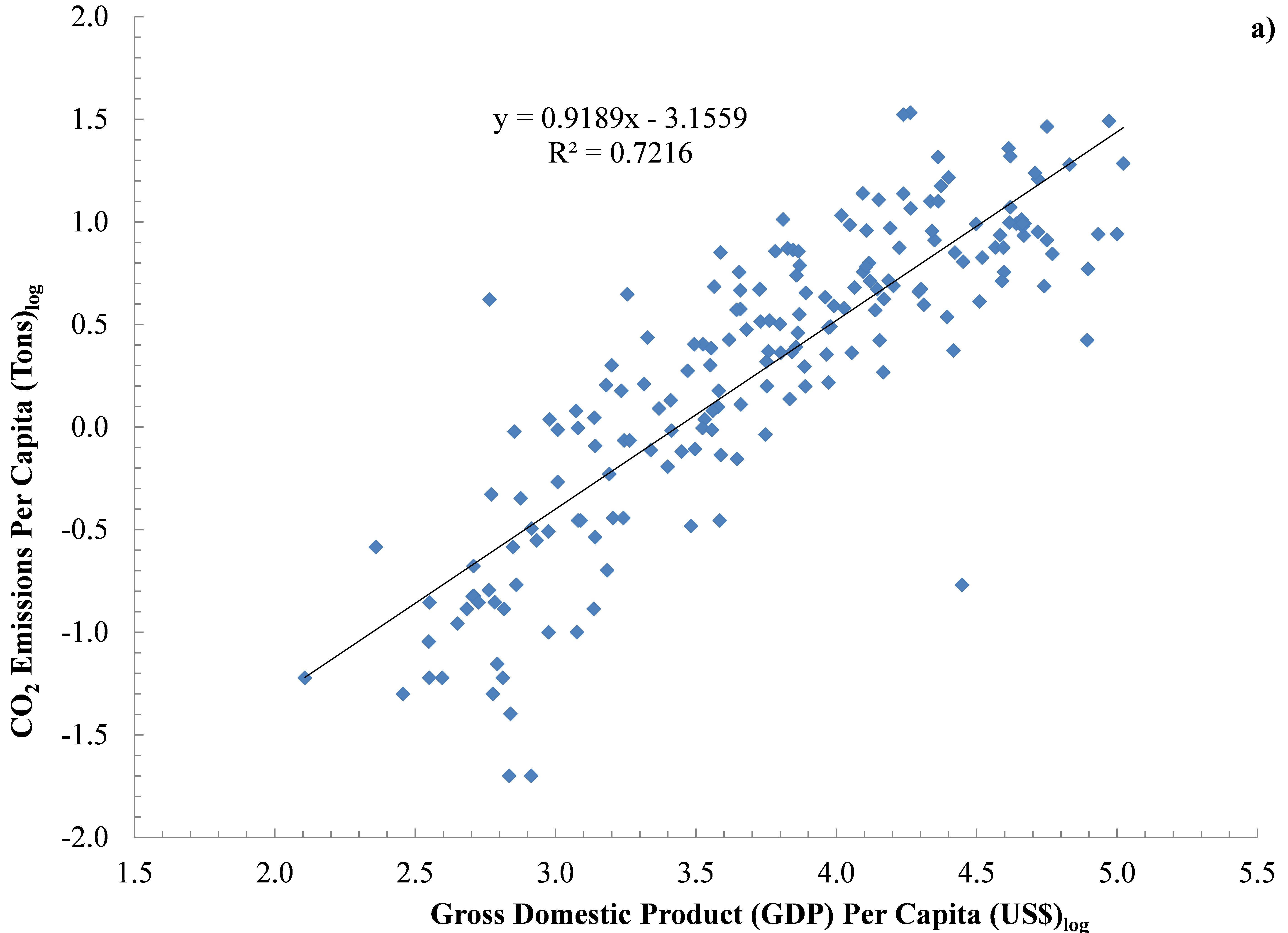
Figure 1a) Global CO2 Per Capita Emissions (Tons) Vs Per Capita Gross Domestic Product (GDP) (US $)
The above regions are ripe for – or currently experiencing – significant political uprisings from the Niger Delta and Venezuela to the percolating anger associated with increasing economic stratification and political elite disconnect in countries like Saudi Arabia, Libya, Yemen, Pakistan, Mediterranean Africa writ large, Sudan, and Oman2. Often this discontent is emanating out of citizens’ concerns as to where oil revenues are going and how often the hydrocarbon largesse is concentrated in a handful of political elites and/or oligarchs (Nossiter, 2014). The EIA estimates Russia and China sit atop an estimated 107 billion barrels of shale oil and 1,400 TCF of shale gas. Much of this resource will be required if they are to continue > 2-5% Gross Domestic Product (GDP) growth. The remainder they will undoubtedly use as a cudgel to deflect the west’s suggestions and/or demands within their borders or their “near abroad.” In the case of Russia, the “near abroad” generally refers to the eight former Communist pliable nations – and are incidentally home to nontrivial shale oil and gas reserves – that act as a physical and ideological buffer between them and NATO/European Union states. In an effort to combat the asymmetric hydrocarbon supply and demand issues and secure access to the sizable shale reserves in eastern Europe, the European Union continues to push the European Neighborhood Policy meant to create a “ring of friends”3 – with Ukraine just the latest significant test and the only successes being Tunisia and Moldova (Charlemagne, 2014). With respect to China, their “near abroad” nations include shale oil and gas rich nations like Indonesia, Thailand, Myanmar, Cambodia, and Vietnam, along with ex-Soviet region Central Asian countries which provide China with 80% of its natural gas needs. However, the east-west tug of war has come down to the willingness of the east to offer larger instant loans, cheaper gas, and labor/technology needed to develop pipeline networks. The nexus between these two eastern giants is the proposed – and recently agreed upon – $400 billion Sino-Russian energy cooperation natural gas and oil pipeline. This proposal will stretch across heretofore relatively undisturbed and isolated communities and the ecosystems they have evolved with across the Eurasian Steppe and Siberia (Einhorn, 2014).
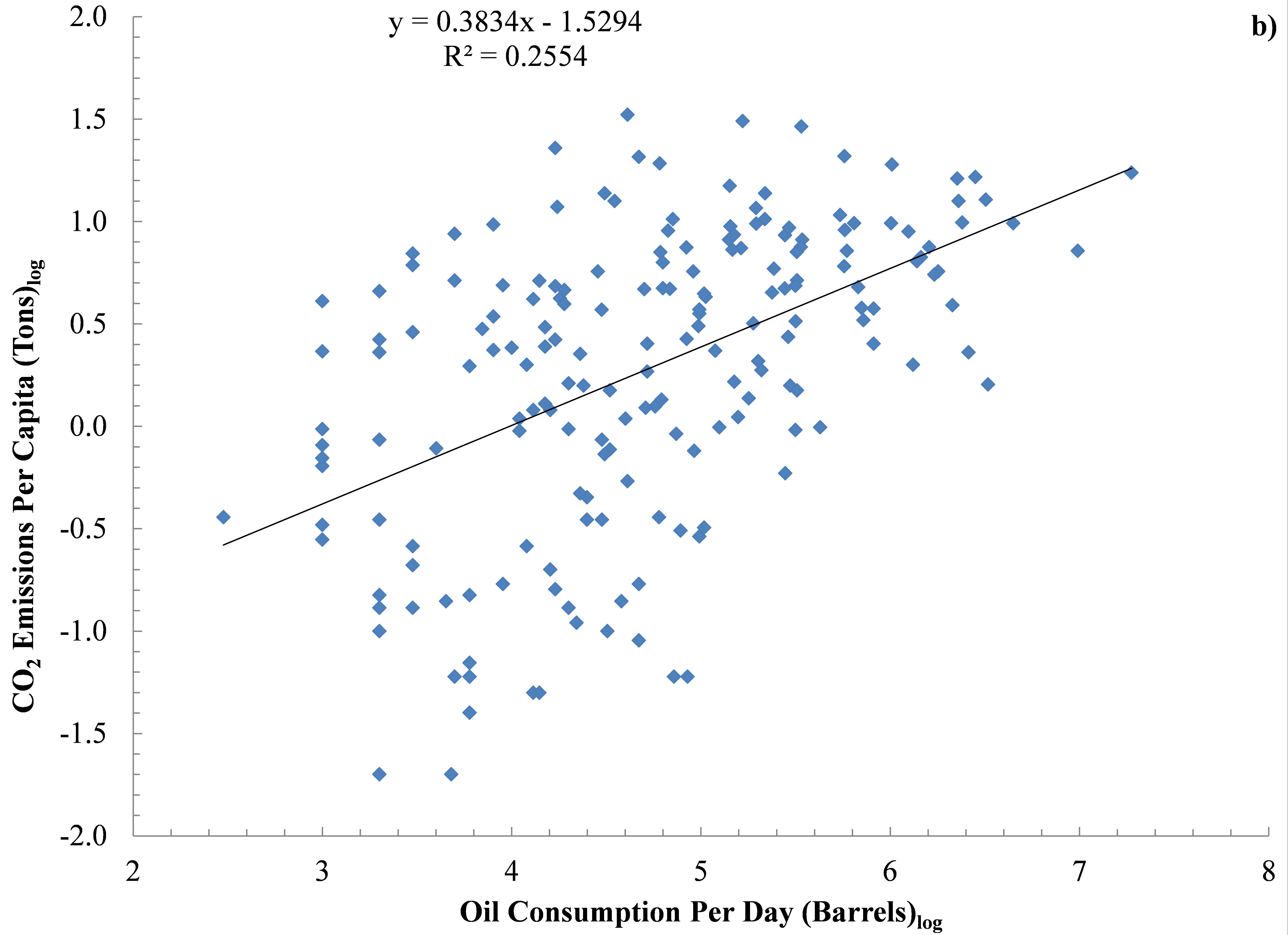
Figure 1b) Global CO2 Per Capita Emissions (Tons) Vs Oil Consumption Per Day (Barrels) across 204 countries
The fomenting anger and geopolitical combativeness that result from these conditions put the global hydrocarbon transport network at risk. Analogies to R.A. Radford’s The Economic Organization of a P.O.W. Camp can be made here, where the economy that Mr. Radford created flourished until the input stream from the Red Cross stopped. It was at this time that the economy collapsed due to its singular reliance on one input source. Similar analogies exist across emerging, P5+1, and frontier markets worldwide, with many countries largely dependent upon hydrocarbon imports or exports to stoke GDP. Such imports, along with oil consumption, account for 98% of per country CO2 emissions (Table 1 below, Figure 1a-b). Revolution or even temporary and targeted political instability will fuel the type of hydrocarbon transport/production disruption that will produce the kind of jump condition described by Mr. Radford. A jump condition occurs in situations when suitable hydrocarbon stocks/flows are lost, pipelines are turned off, and alternative transport channels are deemed too perilous. Such a crisis is one that no industrialized or industrializing nation is prepared to manage, making the 2007-08 Financial Crisis look and feel like child’s play. Thus, many private and state actors are proposing new and expanded hydrocarbon pipeline networks to reduce reliance on single-large networks emanating from or traveling through volatile regions. Proposals range from the large Nabucco pipeline proposal connecting Asia and Europe or the Nord Stream AG Baltic Sea Gas Pipeline to small regional or inter-state proposals in Africa, the Persian Gulf, and Eastern Europe.
The “When?”
With this map, which was initiated in January 2014, we have attempted to accurately quantify as many existing and proposed pipeline routes as possible in Europe, Africa, South America, Asia, and the Persian Gulf. We will be updating this map periodically, and it should be noted that all layers are predetermined aggregations of regional pipelines. Given the recent EIA global shale oil and gas estimates, it is only a matter of time before: a) European nations like Germany, Ukraine, Poland, and Romania begin to explore shale gas extraction in the name of “energy independence,” and b) Argentina hands over the proverbial keys to its 16.2-22.5 billion barrels of oil in the Vaca Muerta shale basin to the likes of Shell or Repsol-YPF (Canty, 2011; Gonzalez and Cancel, 2013; Romero and Krauss, 2013; Staff, 2013). This conversation will be accompanied by additional pipeline proposals for inter- and intra-region transport, all of which we will incorporate into this map on a quarterly basis. If you know of proposals that are not currently shown on the map, please let us know.
Table 1. Major Worldwide Flows of Oil (Thousand Barrels Per Day).
Bordoff, J., 2014. Adding Fuel to the Fire: How the American shale gas boom can weaken Russia’s hand in Ukraine, Foreign Policy Magazine, Washington, DC.
Canty, D., 2011. Repsol hails largest ever 927 million bbl oil find, ArabianOilandGas.com. ITP Business Portal.
Charlemagne, 2014. How to be good neighbours: Ukraine is the biggest test of the EU’s policy towards countries on its borderlands, The Economist, London, UK.
Einhorn, B., 2014. How the Ukraine Crisis Could Help Clear Beijing’s Smog, Bloomberg Businessweek. Bloomberg LP, New York, NY.
Gonzalez, P., Cancel, D., 2013. Shell to Triple Argentine Shale Spending as Winds Change, Bloomberg Magazine. Bloomberg LP, New York, NY.
Gwertzman, B., 2014. How to respond to Ukraine’s Crisis, Council on Foreign Relations, Washington, DC.
Henderson, J., Stern, J., 2014. The Potential Impact on Asia Gas Markets of Russia’s Eastern Gas Strategy, Oxford Energy Comment. The Oxford Institute for Energy Studies, Oxford, UK, p. 13.
Klein, N., 2008. The Shock Doctrine: The Rise of Disaster Capitalism. Picador.
Klein, N., 2014. Why US Fracking Companies Are Licking Their Lips Over Ukraine: From climate change to Crimea, the natural gas industry is supreme at exploiting crisis for private gain – what I call the shock doctrine, The Guardian, London, UK.
Krauss, C., 2014. U.S. Gas Tantalizes Europe, but It’s Not a Quick Fix, The New York Times, New York, NY.
McDonnell, A., 2014. Fracking is unlikely to reduce gas prices to the extent its proponents desire, The London School of Economics and Political Science – British Politics and Policy. The London School of Economics, London, UK.
Nossiter, A., 2014. Nigerians Ask Why Oil Funds Are Missing, The New York Times, New York, NY.
Romero, S., Krauss, C., 2013. An Odd Alliance in Patagonia, The New York Times, New York, NY.
Staff, 2013. Argentina’s YPF: Swallowed Pride, The Economist, London, UK.
Wade, T., Rascoe, A., 2014. Global gas trade may soften foreign policy of Russia, China, Reuters, New York, NY.
[2] The EIA estimates Mediterranean Africa contains 5,772 TCF of estimated wet shale natural gas and 1,373,770 million barrels of oil, the Former Soviet Union 4,738 TCF and 310,567 million barrels, and South America 2,465 TCF and 643,864 million barrels 73% of which is in Brazil and Argentina’s Vaca Muerta.
[3] According to The Economist “The Europeans should also rethink the neighbourhood policy, which lumps together disparate countries merely because they happen to be nearby. In the south it may have to devise a wider concept of its interests stretching out to the Sahel, the Horn of Africa and the Middle East. Here Europe has no real friends, lots of acquaintances and not a few enemies. To the east it needs better ways of helping those who want to move closer to the EU.”
Pipeline spill in Mayflower, AR on March 29, 2013. Photo by US EPA via Wikipedia.
The debate over the Keystone XL pipeline expansion project has grabbed a lot of headlines, but it is just one of several proposed major pipeline projects in the United States. As much of the discussion revolves around potential impacts of the pipeline system, a review of known incidents is relevant to the discussion.
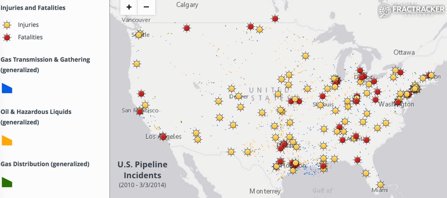
A year ago, the FracTracker Alliance calculated that there was an average of 1.6 pipeline incidents per day in the United Sates. That figure remains accurate, with 2,452 recorded incidents between January 1, 2010 and March 3, 2014, a span of 1,522 days.
The Pipeline and Hazardous Materials Safety Administration (PHMSA) classifies the incidents into three categories:
Gas transmission and gathering: Gathering lines take natural gas from the wells to midstream infrastructure. Transmission lines transport natural gas from the regions in which it is produced to other locations, often thousands of miles away. Since 2010, there have been 486 incidents on these types of lines, resulting in 10 fatalities, 71 injuries, and $620 million in property damage.
Oil and hazardous liquid: This includes all materials overseen by PHMSA other than natural gas, predominantly crude and refined petroleum products. Liquified natural gas is included in this category. There were 1,511 incidents during the reporting period for these pipelines, causing 6 deaths and 15 injuries, and $1.8 billion in property damage.
Gas distribution: These pipelines are used by utilities to get natural gas to consumers. In just over 40 months, there were 455 incidents, resulting in 42 people getting killed, 183 reported injuries, and $86 million in property damage.
Curiously, while incidents on distribution lines accounted for 72 percent of fatalities and 67 percent of all injuries, the property damage in these cases were only responsible for just over 3 percent of $2.5 billion in total property damage from pipeline spills since 2010. A reasonable hypothesis accounting for the deaths and injuries is that distribution lines are much more common in densely populated areas than are the other types of pipelines; an incident that might be fatal in an urban area might go unnoticed for days in more remote locations, for example. However, as the built environment is also much more densely located in urban areas, it does seem surprising that reported property damage isn’t closer to being in line with physical impacts on humans.
How accurate are the data?
In the wake of the events of September 11, 2001, governmental agency data suddenly became much more opaque. In terms of pipelines, public access to the pipeline data that had been mapped to that point was removed. It was later restored, with limitations. As it stands now, most pipeline data in the United States, including the link to the pipeline proposal map above, are intentionally generalized to the point where pipelines might not even be rendered in the appropriate township, let alone street.
There are some exceptions, though. If you would like to know where pipelines are in US waters in the Gulf of Mexcio, for example, the Bureau of Ocean Energy Management makes that data not only accessible to view, but available for download on data.gov, a site dedicated to data transparency. While the PHMSA will not do the same with terrestrial pipelines, the do release location data along with their incident data.
Pipeline incidents from 1/1/2010 through 3/3/2014. To access details, legend, and other map controls, please click the expanding arrows icon in the top-right corner of the map.
This fatal pipeline incident was in Allentown, PA, but was given coordinates in Greenland.
Unfortunately, we see evidence that the data are not well vetted, at least in terms of location. One of the most serious incidents in the timeframe, an explosion in Allentown, Pennsylvania that killed five people and injured three more, was given coordinates that render in the middle of Greenland. Another incident leading to fatalities was given location data that put it in Manatoba, well outside of the reach of the US agency that publishes the data. Still another incident appears to be in the Pacific Ocean, 1,300 miles west-southwest of Mexico. There are many more examples as well, but the majority of incidents seem to be reasonably well located.
Fuzzy data: are national security concerns justified?
Anyone who watches the news on a regular basis knows that there are people out there who mean others harm. However, a closer look at the incident data shows that pipelines are not a common means of accomplishing such an end.
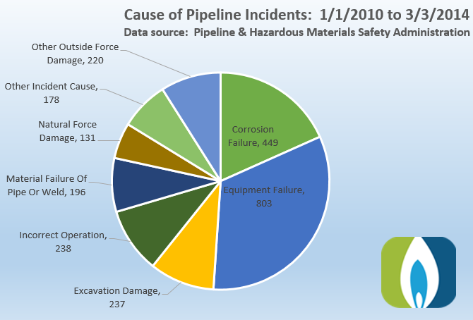
Causes of pipeline incidents from 1/1/10 to 3/3/14, with counts.
For each category showing causation, there are numerous subcategories. While we don’t need to look into all of those here, it is worth pointing out that there is a subcategory of, “other outside force damage” that is designated as, “intentional damage.” Of the 2,452 total incidents, nine incidents fall into this subcategory. These subcategories are further broken down, and while there is an option to express that the incident is a result of terrorism, none have been designated that way in this dataset . Five of the nine incidents are listed as acts of vandalism, however. To be thorough, and because it provides a fascinating insight into work in the field, let’s take a look at the narrative description for each incident that are labeled as intentional in origin:
Approximately 2 bbls of crude oil were released when an unknown person(s) removed the threaded pressure warning device on the scraper trap’s closure door. As a result of the absence of the 1/2 inch pressure warning device crude oil was able to flow from the open port upon start up of the pipeline and pressurization of the scraper trap. Once this was discovered the 1/2 inch pressure warning device was properly put back into the scaper trap.
Aboveground piping intentionally shot by unknown party. Installed stoppall on line at 176+73 (7 146′) upstream of damaged aboveground piping. Cut and capped pipeline.
Friday october 18th at approximately 6:00 p.m. we were notified of a gas line break at Kayenta Mobile Home Park. The Navajo Police responded to an emergency call about vandals in one of the parks alley ways kicking at meters. Upon arrival they found the broke meter riser at the mobile home park and expediently used the emergency shutdown system to remedy the situation. This immediately cut service to 118 customers in the park. [Names removed] responded to the call. we arrived on site at approximately 9:30 p.m. We located the damage and fixed the system at approximately 1:30 a.m. i called the Amerigas emergency call center and informed them that we would be restarting the system the following morning and to tell our customers they would need to be home in order to restore service. We then started the procedure of shutting every valve off to all customers before restarting the system. We started the system back up at 9:30a.m. 10/19/2013. Once the system was up to full pressure and all systems were normal we began putting customers back into service. The completion of re-establishing service to all customers on the system was completed on 10/23/2013.
A service tech was called at 1:15 am Sunday morning to respond to the Marlboro Fire Department at an apparent explosion and house fire. The tech arrived and called for additional resources. He then began to check for migrating gas in the surrounding buildings along the service to the house and in the street. no gas readings were detected. The distribution and service on call personnel arrived and began calling in additional company resources to assist in the response effort and controlling the incident. A distribution crew was called in to shut off and cut the service. Additional service techs were called in to assist in checking the surrounding buildings and in the streets at catch basins and manholes around the entire block. Gas supply personnel were called in and dispatched to take odorant samples in the houses directly across from 15 Grant Ct. that had active gas service. Gas survey crews were called in to survey Grant St. and the two parallel streets McEnelly St. and Washington Ct. along with the portion of Washington st. in between these streets. The meter and meter bar assembly were taken by the investigators as evidence. The service was pressure tested to the riser which was witnessed by a representative of the DPI. The service was cut off at the main. After the investigators completed gathering evidence at the scene they gave permission to begin cleaning up the site. There was a tenant home at the time of the explosion who was conscious and walking around when the fire department arrived. He was taken to the hospital and reports are that he sustained 2nd and 3rd degree burns on portions of his body.
On Friday, September 7, 2012 PSE&G responded to a gas emergency call involving a gas ignition. The initial call came in from the Orange Fire Department at 17:09 as a house fire at 272 Reock Ave Orange; the fire chief stated gas was not involved and the fire was caused by squatters. Subsequent investigation of the incident revealed that the fire was caused when one of the squatters lit a match which ignited leaking gas originating from gas piping removed from the head of an inside meter set. The gas meter inlet valve and associated piping were all removed by an unknown person on an unknown date prior to the fire. An appliance service tech responded and shut the gas off at the curb at 17:40 on September 7 2012. A street crew was dispatched and the gas service to 272 reock ave was cut at the curb at 19:00. Two people (names unknown) squatters were injured one by the fire one was injured jumping out a window to escape the fire. The home in question was vacated by the owner and the injured parties were trespassing on the property at the time of the incident. PSE&G has been unable to confirm any information on the status of their injuries due to patient confidentiality laws.
The homeowner tampered with company piping by removing 3/4″ steel end cap with a 3/4″ steel nipple on the tee was removed which caused the gas leak in the basement and resulted in a flash fire. The most likely source of ignition was the water heater. The homeowner died in the incident.
A structure fire involved an unoccupied hardware store and a small commercial 12-meter manifold. There were no meters on the manifold and no customers lost service. The heat from the structure fire melted a regulator on the manifold which in turn released gas and contributed to the fire. The cause is officially undetermined; however according to the fire department the cause appears to be arson with the fire starting in the back of the building and not from PG&E facilities. PG&E was notified of this incident by the fire department at 1802 hours. The gas service representative arrived on scene at 1830 hours. The fire department stopped the flow of gas by closing the service valve and the fire was extinguished at approximately 1900 hours. this incident was determined to be reportable due to damages to the building exceeding $50,000. There were no fatalities and no injuries as a result of this incident. Local news media was on-site but no major media was present.
A house explosion and fire occurred at approximately 0208 hours on 2/7/10. The fire department called at PG&E at 0213 hours. PG&E personnel arrived at 0245 hours. The fire department had shut off the service valve and removed the meter before PG&E arrived. The house was unoccupied at the time of the explosion. The gas service account was active and the gas service was on (contrary to initial report). The cause of the explosion is undetermined at the time of this report but the fire department has indicated the cause appears to be arson. After the explosion, PG&E performed a leak survey of the service the services on both sides of this address and the gas main in the front of all three of these addresses. No indication of gas was found. PG&E also performed bar hole tests over the service at 3944 17th Avenue and found no indication of gas. The gas service was cut off at the main and will be re-connected when the customer is ready for service.
On Monday, January 25, 2010 at approximately 2:30pm a single-family home at 2022 west 63rd Street Cleveland OH (Cuyahoga County) was involved in an explosion/fire. The gas service line was shut-off at approximately 4:30pm. A leak survey of the main lines and service lines on W. 83rd between Madison and Lorain revealed no indications of gas near the structure. A service leak at 2131 West 83rd Street was detected during the leak survey. This service line was replaced upon discovery. On Tuesday, January 26th, 2010 the service line at 2022 W. 83rd was air tested at operating pressure with no pressure loss. An odor test was conducted at 2028 West 83rd Street. The results of this odor test revealed odor levels well within dot compliance levels. Our investigation revealed an odor complaint at this residence on January 18th. Dominion personnel responded to the call and met with the Cleveland Fire Department. Dominion found the meter disconnected and the meter shut-off valve in the half open position. The shut-off valve was closed by the Dominion technician and secured with a locking device. The technician placed a 3/4 inch plug in the open end of the valve. The technician also attempted to close the curb-slop valve but could not. The service line was then bar hole tested utilizing a combustible gas indicator from the street to the structure. As a result, no leakage was discovered. A second attempt to close the curb box valve on January 19th ended when blockage was discovered in the valve box. The valve box was in the process of being scheduled for excevatlon and shut off by a construction crew at the time of the incident. An investigation of the incident site determined the cause to be arson as approximately 6 inches of service line and the meter shut-off valve (with locking device still intact) detached from the service line were recovered inside the structure.
While several of these narratives do make it seem as if the incidents in question were deliberate, these seem to have been caused by people on the ground, not by some GIS-powered remote effort. Seven of the nine incidents were on distribution lines, which tend to occur in populated areas, where contact with gas infrastructure is in fact commonplace, and six out of those seven incidents occurred inside houses or other structures.
On the other hand, there is a real danger in not knowing where pipelines are located. 237 accidents were due to excavation activities, and 86 others were caused by boats, cars, or other vehicles unrelated to excavation activity. Better knowledge of the location of these pipelines could reduce these numbers significantly.
Water Resource Reporting and Water Footprint from Marcellus Shale Development in West Virginia and Pennsylvania
Report and summary by Meghan Betcher and Evan Hansen, Downstream Strategies; and Dustin Mulvaney, San Jose State University
The use of hydraulic fracturing for natural gas extraction has greatly increased in recent years in the Marcellus Shale. Since the beginning of this shale gas boom, water resources have been a key concern; however, many questions have yet to be answered with a comprehensive analysis. Some of these questions include:
What are sources of water?
How much water is used?
What happens to this water following injection into wells?
With so many unanswered questions, we took on the task of using publically available data to perform a life cycle analysis of water used for hydraulic fracturing in West Virginia and Pennsylvania.
Summary of Findings
Some of our interesting findings are summarized below:
In West Virginia, approximately 5 million gallons of fluid are injected per fractured well, and in Pennsylvania approximately 4.3 million gallons of fluid are injected per fractured well.
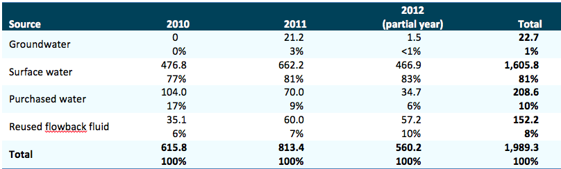
Surface water taken directly from rivers and streams makes up over 80% of the water used in hydraulic fracturing in West Virginia, which is by far the largest source of water for operators. Because most water used in Marcellus operations is withdrawn from surface waters, withdrawals can result in dewatering and severe impacts on small streams and aquatic life.
Most of the water pumped underground—92% in West Virginia and 94% in Pennsylvania—remains there, lost from the hydrologic cycle.
Reused flowback fluid accounts for approximately 8% of water used in West Virginia wells.
Approximately one-third of waste generated in Pennsylvania is reused at other wells.
As Marcellus development has expanded, waste generation has increased. In Pennsylvania, operators reported a total of 613 million gallons of waste, which is approximately a 70% increase in waste generated between 2010 and 2011.
Currently, the three-state region—West Virginia, Pennsylvania, and Ohio—is tightly connected in terms of waste disposal. Almost one-half of flowback fluid recovered in West Virginia is transported out of state. Between 2010 and 2012, 22% of recovered flowback fluid from West Virginia was sent to Pennsylvania, primarily to be reused in other Marcellus operations, and 21% was sent to Ohio, primarily for disposal via underground injection control (UIC) wells. From 2009 through 2011, approximately 5% of total Pennsylvania Marcellus waste was sent to UIC wells in Ohio.
The blue water footprint for hydraulic fracturing represents the volume of water required to produce a given unit of energy—in this case one thousand cubic feet of gas. To produce one thousand cubic feet of gas, West Virginia wells require 1-3 million gallons of water and Pennsylvania wells required 3-4 million gallons of water.
Table 1. Reported water withdrawals for Marcellus wells in West Virginia (million gallons, % of total withdrawals, 2010-2012)
Source: WVDEP (2013a). Note: Surface water includes lakes, ponds, streams, and rivers. The dataset does not specify whether purchased water originates from surface or groundwater. As of August 14, 2013, the Frac Water Reporting Database did not contain any well sites with a withdrawal “begin date” later than October 17, 2012. Given that operators have one year to report to this database, the 2012 data are likely very incomplete.
As expected, we found that the volumes of water used to fracture Marcellus Shale gas wells are substantial, and the quantities of waste generated are significant. While a considerable amount of flowback fluid is now being reused and recycled, the data suggest that it displaces only a small percentage of freshwater withdrawals. West Virginia and Pennsylvania are generally water-rich states, but these findings indicate that extensive hydraulic fracturing operations could have significant impacts on water resources in more arid areas of the country.
While West Virginia and Pennsylvania have recently taken steps to improve data collection and reporting related to gas development, critical gaps persist that prevent researchers, policymakers, and the public from attaining a detailed picture of trends. Given this, it can be assumed that much more water is being withdrawn and more waste is being generated than is reported to state regulatory agencies.
Data Gaps Identified
We encountered numerous data gaps and challenges during our analysis:
All data are self-reported by well operators, and quality assurance and quality control measures by the regulatory agencies are not always thorough.
In West Virginia, operators are only required to report flowback fluid waste volumes. In Pennsylvania, operators are required to report all waste fluid that returns to the surface. Therefore in Pennsylvania, flowback fluid comprises only 38% of the total waste which means that in West Virginia, approximately 62% of their waste is not reported, leaving its fate a mystery.
The Pennsylvania waste disposal database indicates waste volumes that were reused, but it is not possible to determine exactly the origin of this reused fluid.
In West Virginia, withdrawal volumes are reported by well site rather than by the individual well, which makes tracking water from withdrawal location, to well, to waste disposal site very difficult.
Much of the data reported is not publically available in a format that allows researchers to search and compare results across the database. Many operators report injection volumes to FracFocus; however, searching in FracFocus is cumbersome – as it only allows a user to view records for one well at a time in PDF format. Completion reports, required by the Pennsylvania Department of Environmental Protection (PADEP), contain information on water withdrawals but are only available in hard copy at PADEP offices.
In short, the true scale of water impacts can still only be estimated. There needs to be considerable improvements in industry reporting, data collection and sharing, and regulatory enforcement to ensure the data are accurate. The challenge of appropriately handling a growing volume of waste to avoid environmental harm will continue to loom large unless such steps are taken.
https://www.fractracker.org/a5ej20sjfwe/wp-content/uploads/2014/04/GasWellWaterWithdrawals.png732975FracTracker Alliancehttps://www.fractracker.org/a5ej20sjfwe/wp-content/uploads/2025/09/2025-Wordmark-Logo.pngFracTracker Alliance2014-04-04 09:31:062020-07-21 10:42:24Water Use in WV and PA
Data transparency is a major issue in the oil and gas world. Some states in the U.S. do not make the location or other details associated with wells easy to find. If one is looking for Pennsylvania data, however, the basic datasets are quite accessible. The PA Department of Environmental Protection (DEP) maintains several datasets on unconventional drilling activity in the Commonwealth and provides this information online and free of charge to the public. The following databases are ones that we commonly use to update our maps and perform data analyses:
Below are tips for how to search the PA DEP’s records and download datasets if you would like:
Dates
Date ranges must be entered in these databases in order to narrow down the search. We suggest starting with 1/1/2000 through current if you would like to see all unconventional activity to date.
County, Municipality, Region, and Operator
This criteria can be further refined by selecting particular counties, regions, etc.
Unconventional Only
For all datasets, “Unconventional Only – Yes” should be selected if you are only interested in the wells that have been drilled into unconventional shale formations and hydraulically fractured, or “fracked.”
“Unconventional” definitions according to PA Code, Chapter 78:
Unconventional well — A bore hole drilled or being drilled for the purpose of or to be used for the production of natural gas from an unconventional formation.
Unconventional formation — A geological shale formation existing below the base of the Elk Sandstone or its geologic equivalent stratigraphic interval where natural gas generally cannot be produced at economic flow rates or in economic volumes except by vertical or horizontal well bores stimulated by hydraulic fracture treatments or by using multilateral well bores or other techniques to expose more of the formation to the well bore.
Download
Once search criteria have been defined, click View Report to see the most up to date information compiled below. From there, the file can be downloaded in different formats, such as a PDF or Excel file.
Visit this page to see all of the oil and gas reports that the PA DEP issues.
https://www.fractracker.org/a5ej20sjfwe/wp-content/uploads/2014/03/DEP-centered-rgb.png470811FracTracker Alliancehttps://www.fractracker.org/a5ej20sjfwe/wp-content/uploads/2025/09/2025-Wordmark-Logo.pngFracTracker Alliance2014-03-28 10:03:252020-07-21 10:42:24Finding PA Department of Environmental Protection Data
By Ted Auch, PhD – OH Program Coordinator, FracTracker Alliance
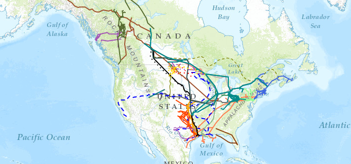
With all the focus on the existing TransCanada Keystone XL pipeline – as well as the primary expansion proposal recently rejected by Lancaster County, NB Judge Stephanie Stacy and more recently the Canadian National Energy Board’s approval of Enbridge’s Line 9 pipeline – we thought it would be good to generate a map that displays related proposals in the US and Canada.
North American Proposed Pipelines and Current Pipelines
To view the fullscreen version of this map along with a legend and more details, click on the arrows in the upper right hand corner of the map.
The map was last updated in October 2014.
Pipeline Incidents
The frequency and intensity of proposals and/or expansions of existing pipelines has increased in recent years to accompany the expansion of the shale gas boom in the Great Plains, Midwest, and the Athabasca Tar Sands in Alberta. This expansion of existing pipeline infrastructure and increased transport volume pressures has resulted in significant leakages in places like Marshall, MI along the Kalamazoo River and Mayflower, AR. Additionally, the demand for pipelines is rapidly outstripping supply – as can be seen from recent political pressure and headline-grabbing rail explosions in Lac-Mégantic, QC, Casselton, ND, Demopolis, AL, and Philadelphia.1 According to rail transport consultant Anthony Hatch, “Quebec shocked the industry…the consequences of any accident are rising.” This sentiment is ubiquitous in the US and north of the border, especially in Quebec where the sites, sounds, and casualties of Lac-Mégantic will not soon be forgotten.
Improving Safety Through Transparency
It is imperative that we begin to make pipeline data available to all manner of parties ex ante for planning purposes. The only source of pipeline data historically has been the EIA’s Pipeline Network. However, the last significant update to this data was 7/28/2011 – meaning much of the recent activity has been undocumented and/or mapped in any meaningful way. The EIA (and others) claims national security is a primary reason for the lack of data updates, but it could be argued that citizens’ right-to-know with respect to pending proposals outweighs such concerns – at least at the county or community level. There is no doubt that pipelines are magnets for attention, stretching from the nefarious to the curious. Our interest lies in filling a crucial and much requested data gap.
Metadata
Pipelines in the map above range from the larger Keystone and Bluegrass across PA, OH, and KY to smaller ones like the Rex Energy Seneca Extension in Southeast Ohio or the Addison Natural Gas Project in Vermont. In total the pipeline proposals presented herein are equivalent to 46% of EIA’s 34,133 pipeline segment inventory (Table 1).
Table 1. Pipeline segments (#), min/max length, total length, and mean length (miles).
Section
#
Min
Max
Mean
Sum
Bakken
34
18
560
140
4,774
MW East-West
68
5
1,056
300
20,398
Midwest to OK/TX
13
13
1,346
307
3,997
Great Lakes
5
32
1,515
707
3,535
TransCanada
3
612
2,626
1,341
4,021
Liquids Ventures
2
433
590
512
1,023
Alliance et al
3
439
584
527
1,580
Rocky Express
2
247
2,124
1,186
2,371
Overland Pass
6
66
1,685
639
3,839
TX Eastern
15
53
1,755
397
5,958
Keystone Laterals
4
32
917
505
2,020
Gulf Stream
2
541
621
581
1,162
Arbuckle ECHO
25
27
668
217
5,427
Sterling
9
42
793
313
2,817
West TX Gateway
13
1
759
142
1,852
SXL in PA and NY
15
48
461
191
2,864
New England
70
2
855
65
4,581
Spectra BC
9
11
699
302
2,714
Alliance et al
4
69
4,358
2,186
4,358
MarkWest
63
2
113
19
1,196
Mackenzie
46
3
2,551
190
8,745
Total
411
128
1,268
512
89,232†
† This is equivalent to 46% of the current hydrocarbon pipeline inventory in the US across the EIA’s inventory of 34,133 pipeline segments with a total length of 195,990 miles
The map depicts all of the following (Note: Updated quarterly or when notified of proposals by concerned citizens):
We generated this map by importing JPEGs into ArcMAP 10.2, we then “Fit To Display”. Once this was accomplished we anchored the image (i.e., georeferenced) in place using a minimum of 10 control points (Note: All Root Mean Square (RMS) error reports are available upon request) and as many as 30-40. When JPEGs were overly distorted we then converted or sought out Portable Network Graphic (PNG) imagery to facilitate more accurate anchoring of imagery.
We will be updating this map periodically, and it should be noted that all layers are a priori aggregations of regional pipelines across the 4 categories above.
Every six months, the Pennsylvania Department of Environmental Protection (PADEP) publishes production and waste data for all unconventional wells drilled in the Commonwealth. These data are self-reported by the industry to PADEP, and in the past, there have been numerous issues with the data not being reported in a timely fashion. Therefore, the early versions of these two datasets are often incomplete. For that reason, I now like to wait a few weeks before analyzing and mapping this data, so as to avoid false conclusions. That time has now come.
This map contains production and waste totals from unconventional wells in Pennsylvania from July to December, 2013. Based on data downloaded March 6, 2014. Also included are facilities that received the waste produced by these wells. To access the legend and other map controls, please click the expanding arrows icon at the top-right corner of the map.
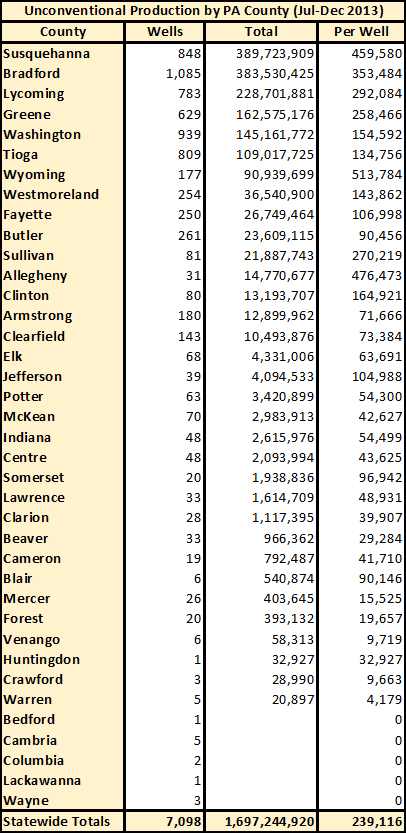
Production
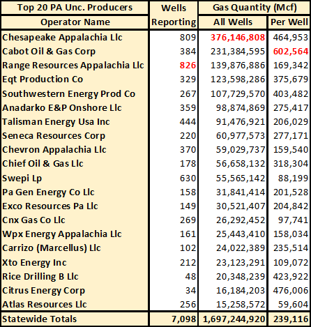
Table 1: Top 20 unconventional gas producers in PA, from July to December 2013. Highest values in each column are highlighted in red.
Production values can be summarized in many ways. In this post, we will summarize the data, first by operator, then by county. For operators, we will take a look at all operators on the production report, and see which operator has the highest total production, as well as production per well (Table 1).
It is important to note that not all of the wells on the report are actually in production, and not all of the ones that are produce for the entire cycle. However, there is some dramatic variance in the production that one might expect from an unconventional well in Pennsylvania that correlates strongly with which operator drilled the well in question. For example, the average Cabot well produces ten times the gas that the average Atlas well does. Even among the top two producers, the average Chesapeake well produces 2.75 times as much as the average Range Resources well.
The location of the well is the primary factor in regards to production values. 74 percent of Atlas’ wells are in Greene and Fayette counties, in southwestern Pennsylvania, while 99 percent of Cabot’s wells are in Susquehanna County. Similarly, 79 percent of Range Resources’ wells are in the its southwestern PA stronghold of Washington County, while 62 percent of Chesapeake’s wells are in Bradford county, in the northeast.
Table 2: PA unconventional gas production by county, from July to December 2013
Altogether, there are unconventional wells drilled in 38 Pennsylvania counties, 33 of which have wells that are producing (see Table 2). And yet, fully 1 trillion cubic feet (Tcf) of t he 1.7 Tcf produced by unconventional wells during the six month period in Pennsylvania came from the three northeastern counties of Susquehanna, Bradford, and Lycoming.
While production in Greene County does not compare to production in Susquehanna, this disparity still does not account for the really poor production of Atlas wells, as that operator averages less than one fourth of the typical well in the county. Nor can we blame the problem on inactive wells, as 84 of their 85 wells in Greene County are listed as being in production. There is an explanation, however. All of these Atlas wells were drilled from 2006 through early 2010, so none of them are in the peak of their production life cycles.
There is a different story in Allegheny County, which has a surprising high per well yield for a county in the southwestern part of the state. Here, all of the wells on the report were drilled between 2008 and 2013, and are therefore in the most productive part of the well’s life cycle. Only the most recent of these wells is listed as not being in production.
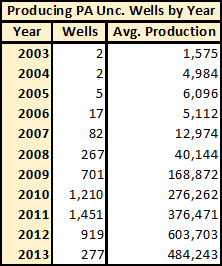
Table 3: Per well production during last half of 2013 for PA unconventional wells by spud year
Generally speaking, the further back a well was originally drilled, the less gas it will produce (see Table 3). At first glance, it might be surprising to note that the wells drilled in 2012 produced more gas than those drilled in 2013, however, as the data period is for the last half of 2013, there were a number of wells drilled that year that were not in production for the entire data cycle.
In addition to gas, there were 1,649,699 barrels of condensate and 182,636 barrels of oil produced by unconventional wells in Pennsylvania during the six month period. The vast majority of both of these resources were extracted from Washington County, in the southwestern part of the state. 540 wells reported condensate production, while 12 wells reported oil.
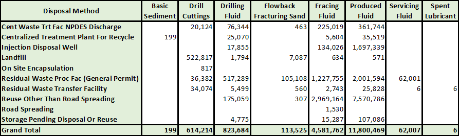
Waste
There are eight types of waste detailed in the Pennsylvania data, including:
Basic Sediment (Barrels) – Impurities that accompany the desired product
Drill Cuttings (Tons) – Broken bits of rock produced during the drilling process
Flowback Fracturing Sand (Tons) – Sand used as proppants during hydraulic fracturing that return to the surface
Fracing Fluid Waste (Barrels) – Fluid pumped into the well for hydraulic fracturing that returns to the surface. This includes chemicals that were added to the well.
Produced Fluid (Barrels) – Naturally occurring brines encountered during drilling that contain various contaminants, which are often toxic or radioactive
Servicing Fluid (Barrels) – Various other fluids used in the drilling process
Spent Lubricant (Barrels) – Oils used in engines as lubricants
Table 4: Method of disposing of waste generated from unconventional wells in PA from July to December 2013
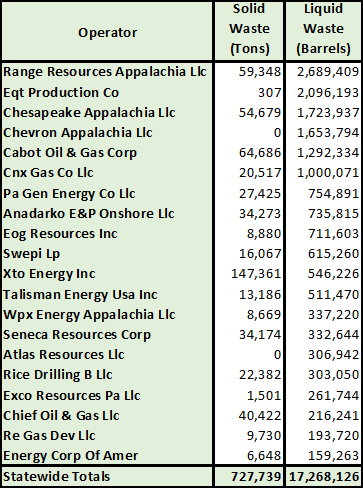
Table 5: Solid & liquid waste disposal for top 20 producers of PA unconventional liquid waste during last half of 2013
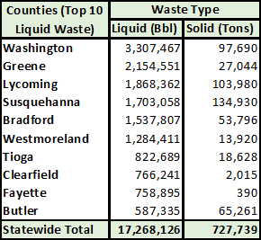
Table 6: Solid & liquid waste totals for the 10 counties that produced the most liquid waste over the 6 month period
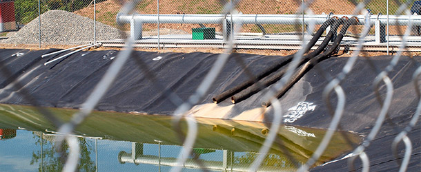
There are numerous methods for disposing of drilling waste in Pennsylvania (see Table 4). Some of the categories include recycling for future use, others are merely designated as stored temporarily, and others are disposed or treated at a designated facility. One of the bright points of the state’s waste data is that it includes the destination of that waste on a per well basis, which has allowed us to add receiving facilities to the map at the top of the page.
As eight data columns per table is a bit unwieldy, we have aggregated the types by whether they are solid (reported in tons) or liquid (reported in 42 gallon barrels). Because solid waste is produced as a result of the drilling and fracturing phases, it isn’t surprising that the old Atlas wells produced no new solid waste (see Table 5). Chevron Appalachia is more surprising, however, as the company spudded 46 wells in 2013, 12 of which were started during the last half of the year. However, Chevron’s liquid waste totals were significant, so it is possible that some of their solid waste was reported, but miscategorized.
As with production, location matters when it comes to the generation of waste from these wells. But while the largest gas producing counties were led by three counties in the northeast, liquid waste production is most prolific in the southwest (see Table 6).
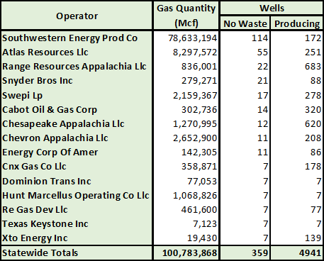
Table 7: PA unconventional operators with the most wells that produced gas, oil, and/or condensate, but no amount of waste.
Finally, we will take a look at the 359 wells that are indicated as in production, yet were not represented on the waste report as of March 6th. These remarkable wells are run by 38 different operators, but some companies are luckier with the waste-free wells than their rivals. As there was a six-way tie for 10th place among these operators, as sorted by the number or wells that produce gas, condensate, or oil but not waste, we can take a look at the top 15 operators in this category (see Table 7). Of note, gas quantity only includes production from these wells. Column on the right shows total number of wells that are indicated as producing, for that same operator, regardless of waste production.
114 of Southwestern Energy’s 172 producing wells were not represented on the waste report as of March 6th, representing just under two thirds of the total. In terms of the number of waste-free wells, Atlas was second, with 55. As for the highest percentage, Dominon, Hunt, and Texas Keystone all managed to avoid producing any waste at all for each of their seven respective producing wells, according to this self-reported data.
https://www.fractracker.org/a5ej20sjfwe/wp-content/uploads/2013/10/Impoundment.jpg250610Matt Kelso, BAhttps://www.fractracker.org/a5ej20sjfwe/wp-content/uploads/2025/09/2025-Wordmark-Logo.pngMatt Kelso, BA2014-03-13 14:33:502020-07-21 10:42:22PA Production and Waste Data Updated
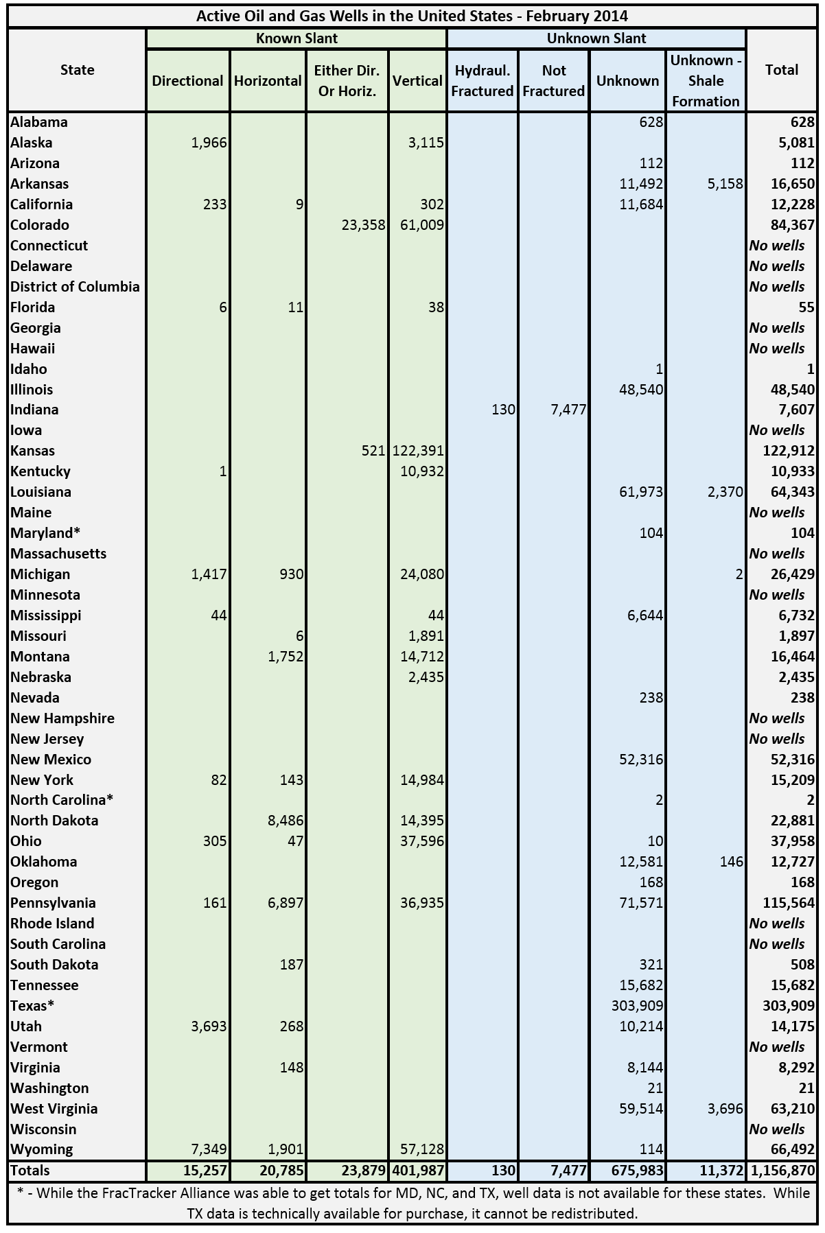
Many people ask us how many wells have been hydraulically fractured in the United States. It is an excellent question, but not one that is easily answered; most states don’t release data on well stimulation activities. Also, since the data are released by state regulatory agencies, it is necessary to obtain data from each state that has oil and gas data to even begin the conversation. We’ve finally had a chance to complete that task, and have been able to aggregate the following totals:
Oil and gas summary data of drilled wells in the United States.
While data on hydraulically fractured wells is rarely made available, the slant of the wells are often made accessible. The well types are as follows:
Directional: Directional wells are those where the top and the bottom of the holes do not line up vertically. In some cases, the deviation is fairly slight. These are also known as deviated or slant wells.
Horizontal: Horizontal wells are directional wells, where the well bore makes something of an “L” shape. States may have their own definition for horizontal wells. In Alaska, these wells are defined as those deviating at least 80° from vertical. Currently, operators are able to drill horizontally for several miles.
Directional or Horizontal: These wells are known to be directional, but whether they are classified as horizontal or not could not be determined from the available data. In many cases, the directionality was determined by the presence of directional sidetrack codes in the well’s API number.
Vertical: Wells in which the top hole and bottom hole locations are in alignment. States may have differing tolerances for what constitutes a vertical well, as opposed to directional.
Hydraulically Fractured: As each state releases data differently, it wasn’t always possible to get consistent data. These wells are known to be hydraulically fractured, but the slant of the well is unknown.
Not Fractured: These wells have not been hydraulically fractured, and the slant of the well is unknown.
Unknown: Nothing is known about the slant, stimulation, or target formation of the well in question.
Unknown (Shale Formation): Nothing is known about the slant or stimulation of the wells in question; however, it is known that the target formation is a major shale play. Therefore, it is probable that the well has been hydraulically fractured, with a strong possibility of being drilled horizontally.
Wells that have been hydraulically fractured might appear in any of the eight categories, with the obvious exception of “Not Fractured.” Categories that are very likely to be fractured include, “Horizontal”, “Hydraulically Fractured”, and “Unknown (Shale Formation),” the total of which is about 32,000 wells. However, that number doesn’t include any wells from Texas or Colorado, where we know thousands wells have been drilled into major shale formations, but the data had to be placed into categories that were more vague.
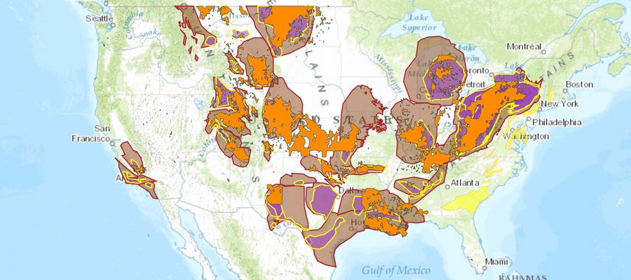
Oil and gas wells in the United States, as of February 2014. Location data were not available for Maryland (n=104), North Carolina (n=2), and Texas (n=303,909). To access the legend and other map tools, click the expanding arrows icon in the top-right corner.
The standard that we attempted to reach for all of the well totals was for wells that have been drilled but have not yet been plugged, which is a broad spectrum of the well’s life-cycle. In some cases, decisions had to be made in terms of which wells to include, due to imperfect metadata.
No location data were available for Maryland, North Carolina, or Texas. The first two have very few wells, and officials in Maryland said that they expect to have the data available within about a month. Texas location data is available for purchase, however such data cannot be redistributed, so it was not included on the map.
It should not be assumed that all of the wells that are shown in the map above the shale plays and shale basin layers are actually drilled into shale. In many cases, however, shale is considered a source rock, where hydrocarbons are developed, before the oil and gas products migrate upward into shallower, more conventional formations.
The raw data oil and gas data is available for download on our site in shapefile format.
https://www.fractracker.org/a5ej20sjfwe/wp-content/uploads/2014/03/US-ShaleViewer-Feature.jpg400900Matt Kelso, BAhttps://www.fractracker.org/a5ej20sjfwe/wp-content/uploads/2025/09/2025-Wordmark-Logo.pngMatt Kelso, BA2014-03-04 12:37:152020-07-21 10:41:55Over 1.1 Million Active Oil and Gas Wells in the US
By Thomas DiPaolo, 2013 GIS Intern, FracTracker Alliance
ND Shale Viewer
Out of North Dakota’s 53 counties, 19 are responsible for producing the oil and natural gas that has brought the state so much prosperity and attention. It’s the latest get-rich-quick scheme, and one that works better than that name would suggest: drive to North Dakota, work in the oil fields for six months, and go home with enough money to find something more permanent. This means that some of the quiet towns overlying the Bakken formation are exploding in size, and many of their new residents lack any connection to these communities when they’re off duty. In the past, similar population booms have been tied to a corresponding increase in crime rates and drug usage, and FracTracker Alliance has examined the available data to find out how much life has changed in North Dakota since the oil started to flow.
Housing Availability
There’s a reason why the you have to drive to North Dakota if you want to stay in the black, and it helps if you’ve got a comfortable car.
Perhaps the biggest problem here, perhaps a cause of others, is that there is simply not enough housing for everyone who wants to work in North Dakota. Trailer parks pack every available inch of space for families from out of state prepared to settle in, becoming themselves towns in miniature, and one of the benefits to consider when working for one oil drilling company over another is to find out which ones are constructing dedicated worker housing and amenities. Familiarity doesn’t fail to breed contempt; demand for living space is so high, in fact, that families who have lived in these towns their whole lives are being forced out as rent prices rise without end. Meanwhile, many have taken to simply sleeping in their cars, and tensions have grown as stores forbid them from parking overnight in their lots.
Crime
With the number of people moving into the state to work in the oil fields, or in industries that support them, North Dakota’s population reached 699,628 in 2012, a jump from the 642,200 people of 2000. More people, of course, means greater effort required to keep the peace – The number of law enforcement officers accordingly jumped from 967 in 2000 to 1,253 in 2012. At first glance, one might think that did the job, since the crime rate fell from 2,203 index crimes1 reported per 100,000 people to 2,122 per 100,000 people, and the number of arrests per officer stayed constant (3.1 in 2000, 3.0 in 2012). That conclusion doesn’t hold up well when you look at how crime has fluctuated within the oil-producing counties.2 The population there has risen to 183,940 people, from just 167,515 people in 2000, and it currently employs 379 law enforcement officers, up from 250 officers. In 2000 the crime rate was already in excess of the state average at 1,582 index crimes reported per 100,000 people and 8.3 arrests per law enforcement officer. By 2012, those figures reached 1,629 crimes per 100,000 people and 12.8 arrests per officer. With only a quarter of the state’s population, the crime rate is three-quarters of the state average. This upswell applies especially to violent crimes. Violent crime reports, numbered at 558 statewide in 2000, nearly tripled to 1,445 in 2012; in the oil counties, they more than tripled from 103 to 363 crimes reported. That number carries through in the crime rate figures; statewide, 206.5 violent crimes occurred per 100,000 people in 2012, while only 86.9 crimes were reported per 100,000 people in 2000; in the oil counties, 197.3 violent crimes were reported per 100,000 people in 2012, compared to only 61.5 violent crimes per 100,000 people in 2000. See Table 1 for a comparison of total and violent crimes between the year 2000 and the year 2012.
Table 1. Crime rates per 100,000 people in North Dakota (2000 vs. 2012)
Total Index Crimes
Violent Crimes
Statewide
Oil Counties
Statewide
Oil Counties
2000
2,203
1,582
86.9
61.5
2012
2,122
1,629
206.5
197.3
Where the line blurs is in addressing property crime. Until 2009, there had been a steady decline in the rate of property crime. Since then, however, it has been increasing every year, even if the 2012 figures are still beneath those of 2000. Statewide, the number of property crimes hovered at 13,592 reported crimes in 2000 and 13,402 in 2012, while in the oil counties they rose slightly from 2,547 property crimes in 2000 to 2,634 crimes in 2012. At the same time, the property crime rates fell both statewide (2,116 crimes per 100,000 people to 1,916 per 100,000 people) and in the oil counties (1,529 crimes per 100,000 people to 1,486 per 1000,000 people).
Prostitution
When you have that many single young men together, as so many of the oil field workers are, a market inevitably springs up for very particular crimes. Prostitution stings consume a greater quantity of police time than ever before, with some ND counties reporting their first prostitution arrests ever. In many cases, the suspects in these cases demonstrate a similar attitude to the oil workers they court: stay for a brief period (typically days rather than months), make enough money to support themselves, and keep going out of town. Officers often say that these cases are risky, as they require enough evidence to prove the intent of both parties to exchange money for sex. Without an undercover officer to carry out a sting, many cases could be accused of discrimination, especially in cases where race may be an issue. In other situations, sting operations have provided evidence of drug activity in addition to prostitution.
Drug Use
Juvenile Alcohol Use
In addition to the oil boom, North Dakota has the uncomfortable claim of being one of the nation’s leaders when it comes to binge drinking. It’s notable then to see that, while juvenile3 alcohol use has fallen drastically across the board, juveniles are developing more permissive attitudes towards alcohol use. Between 2000 and 2011, the number of juveniles who reported using alcohol within the previous month fell from 18,000 to 7,000, and it fell from 11,000 to 4,000 juveniles in regards to binge drinking4 on a weekly basis. At the same time, the number of juveniles showing signs of alcohol dependence or abuse fell from 6,000 to 2,000, and those described as needing but not receiving treatment for alcohol abuse fell from 5,000 to 2,000. Yet only 17,000 juveniles reported perceiving great risk from said binge drinking in 2011, where 22,000 had reported perceiving great risk in 2000. Why are more juveniles rejecting personal alcohol use while becoming less concerned with others’ usage?
Adult Drug & Alcohol Use
Whatever the reason, adult alcohol usage has demonstrated the opposite trend: more people are drinking but fewer enjoy it. Between 2000 and 2011, the number of adults using alcohol monthly rose from 286,000 to 320,000, and those binge drinking weekly rose from 144,000 to 165,000. The number of adults perceiving great risk from weekly binge drinking also rose from 173,000 to 183,000, but the number with signs of alcohol dependence or abuse rose from 33,000 to 47,000. Interestingly, the number of adults described as needing but not receiving treatment for alcohol use has barely changed in this time; 46,000 adults were characterized this way in 2000, as opposed to 45,000 of them in 2011.
Smoking and Marijuana Use
The one trend shared between both juveniles and adults is a steady increase in the number of people expressing permissive attitudes towards the use of marijuana. In 2000, 4,000 juveniles and 13,000 adults reported using marijuana within the previous month; by 2011, only 2,000 juveniles reported using marijuana within the previous month, but the number of adults doing so had jumped to 23,000. At that time, only 17,000 juveniles and 171,000 adults reported perceiving great risk from the use of marijuana on a monthly basis, down from 25,000 and 213,000 respectively in 2000. These figures come at a time when other forms of smoking are becoming less popular across the U.S. In 2000 in ND, 16,000 juveniles were using tobacco products on a monthly basis, and 13,000 were using cigarettes specifically; those numbers had fallen to 6,000 and 5,000 juveniles respectively by 2000. Even among adults there were small declines over this time period: 154,000 adults were using tobacco monthly in 2011 as opposed to 161,000 in 2000, and 121,000 adults as opposed to 128,000 were using cigarettes. And while the number of juveniles perceiving great risk from pack-a-day smoking fell from 38,000 to 32,000 between 2000 and 2011, while 346,000 adults perceived great risk from it in 2011, as opposed to 315,000 in 2000.
Footnotes
According to the Crime and Homicide Reports of the North Dakota Attorney General’s office, index crimes are reported to the National Uniform Crime Reporting program managed by the Federal Bureau of Investigation in order to broadly describe the level of criminal activity around the country. They are divided into two categories, violent and property-related. The violent index crimes tracked by North Dakota are murder and non-negligent manslaughter, forcible rape, robbery, and aggravated assault. The property index crimes tracked by the state are burglary, larceny and theft, and motor vehicle theft.
The North Dakota Association of Oil and Gas Producing Counties lists the following counties as its members: Adams, Billings, Bottineau, Bowman, Burke, Divide, Dunn, Golden Valley, Hettinger, McHenry, McKenzie, McLean, Mercer, Mountrail, Renville, Slope, Stark, Ward, and Williams.
The National Surveys on Drug Use and Health define a “juvenile” as any person between the ages of 12 and 17 years, and an adult as any person aged 18 years or older.
The National Surveys on Drug Use and Health define “binge drinking” as consuming five or more alcoholic beverages in one sitting.
https://www.fractracker.org/a5ej20sjfwe/wp-content/uploads/2014/02/Screen-Shot-2014-02-05-at-10.16.56-AM-e1426104364870.png259648Guest Authorhttps://www.fractracker.org/a5ej20sjfwe/wp-content/uploads/2025/09/2025-Wordmark-Logo.pngGuest Author2014-02-07 13:01:512020-07-21 10:41:53Oil Drilling’s Impact on ND Communities
Our latest Ohio-focused map shows the many companies involved in directional drilling in the state and the contact information for these firms.
Layer Descriptions
1. UNIVERSAL WELL SERVICES
Universal Well Services Inc. is a major firm involved in all manner of directional drilling services with an office in Wooster, OH, one in Allen, KY, six in Pennsylvania, six in Texas, and one in West Virginia
2. LLC & MLP’s
This is an inventory of 410 Ohio directional drilling affiliated LLC and MLP firms and contact information. Seventy-eight percent of these firms are domiciled in Ohio. The other primary states that house these firms are Pennsylvania (22), Texas (23), and West Virginia (9). The Economist wrote of these types of firms:
The move away from the C corporation began in earnest in 1975. Wyoming, that vibrant business hub, adopted a new entity structure, the limited-liability company (LLC). Imported from Panama, it provided the tax treatment of a partnership while preserving the corporate protection from individual liability for company debts and litigation. Other states followed in adopting the model. Businesses were quick to see the advantages. The various new types of firm that have risen in the wake of the LLC… make similar use of partnership structures. They have tended to be industry- or sector-specific, at least to begin with. The energy business has a lot of MLPs not only because it needs capital but because it is an easy place to set them up: since 1987, tax law has allowed “mineral or natural resource” companies to operate as listed partnerships, while withholding that privilege from others. But as with other pass-through structures, the constraints are being lowered and circumvented.
3. DRILLING FIRMS
This is an inventory of 393 Ohio Department of Natural Resources permitted directional and injection drilling firms with single locations and their contact information. Seventy-six percent of these firms are domiciled in Ohio with the other primary states of incorporation being Pennsylvania (15), Texas (14), Michigan (11), and West Virginia (9). Only 3 of these firms listed in the Ohio RBDMS Microsoft Access Database contained correct contact information or addresses. According to ODNR staff – and primary FOIA contact:
… it looks like the [active drillers] list [doesn’t contain] much information on the companies in general…We have mailing information for the operating companies, but a lot of the time they subcontract out to get their drillers. We do not require the information of the drillers they contract.
4. ADDITIONAL DRILLERS
This is an inventory of the 40 known locations for six firms permitted to drill in Ohio. The same lack of contact and address data for these firms were true for this data. The primary firms are Butch’s Rathole and Nomac Drilling Corporation. Given that the ODNR RBDMS does not indicate the actual location from which these companies migrated into the Ohio shale industry we decided to include all known locations for these firms.
5. CANADIAN FIRMS
This is an inventory of the 14 known locations for the 5 Canadian drilling firms permitted in Ohio. The primary firm is Savannah Drilling, which is composed of 10 locations across Alberta and Saskatchewan.
6. AMERICAN SUPPORTING CO.
This is an inventory of 1,837 Ohio energy firms operating in the Utica and Marcellus shale or servicing it in a secondary or tertiary fashion. Seventy-five percent (1,386) of these firms are domiciled in Ohio with secondary hotspots in Texas (76), West Virginia (65), Pennsylvania (49), Michigan (34), Colorado (27), Illinois (22), Oklahoma (21), California (16), New York and New Jersey (27), Kentucky (14).
7. ADDITIONAL SUPPORTING CO.
This shows an inventory of 10 Ohio energy firms operating in the Utica and Marcellus shale or servicing it in a secondary or tertiary fashion extracted from the ODNR RBDMS that did not contain locational or contact information.
8. CANADIAN SUPPORTING CO.
This is an inventory of 5 (1 company Mar Oil Company was not found) Canadian energy firms operating in the Utica and Marcellus shale or servicing it in a secondary or tertiary fashion.
9. BRINE HAULERS
This is an inventory of 505 ODNR permitted brine haulers active in the transport and disposal of hydraulic fracturing waste either via injection or waste landfill disposal. Seventy-six percent of these firms are domiciled in Ohio with the primary cities being Zanesville (18), Cambridge, Wooster, and Millersburg (12 each), Canton and Marietta (11 each), Columbus (9), Jefferson (9), Logan (8), and North Canton and Newark (7 each). Pennsylvania and West Virginia are home to 84 and 32 brine haulers, respectively.
https://www.fractracker.org/a5ej20sjfwe/wp-content/uploads/2014/02/Screen-Shot-2014-02-06-at-12.22.35-PM.png324696Ted Auch, PhDhttps://www.fractracker.org/a5ej20sjfwe/wp-content/uploads/2025/09/2025-Wordmark-Logo.pngTed Auch, PhD2014-02-06 10:24:172020-07-21 10:41:53Ohio Production and Injection Well Firms Map


 The use of hydraulic fracturing for natural gas extraction has greatly increased in recent years in the Marcellus Shale. Since the beginning of this shale gas boom, water resources have been a key concern; however, many questions have yet to be answered with a comprehensive analysis. Some of these questions include: