Mapping California’s State Bill 4 (SB4) Well Stimulation Notices
By Kyle Ferrar, CA Program Coordinator, FracTracker Alliance
Introduction
California passed State Bill 4 (SB4) in September, 2013 to develop and establish a regulatory structure for unconventional resource extraction (hydraulic fracturing, acidizing, and other stimulation techniques) for the state. As a feature of the current version of the regulations, oil and gas drilling/development operators are required to notify the California Department of Conservation’s Division of Oil Gas and Geothermal Resources (DOGGR), as well as neighboring property owners, 30 days prior to stimulating an oil or gas well. In addition to property owners having the right to request baseline water sampling within the the following 20 days, DOGGR posts the well stimulation notices to their website.
Current State of Oil and Gas Production
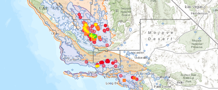
The DOGGR dataset of well stimulation notices was downloaded, mapped, the dataset explored, and well-site proximity to certain sites of interest were evaluated using GIS techniques. First, the newest set of well stimulation notices, posted 1/17/14 were compared to a previous version of the same dataset, downloaded 12/27/13. When the two datasets are compared there are several distinct differences. The new dataset has an additional field identifying the date of permit approval and fields for latitude/longitude coordinates. This is an improvement, but there is much more data collected in the DOGGR stimulation notification forms that can be provided digitally in the dataset, including sources of water, amount of water used for stimulation, disposal methods, etc… An additional 60 wells have been added to the dataset, making the total count now 249 stimulation notices, with 37 stimulated by acid matrix (acidizing), 212 hydraulically fractured, and 3 by both. Of the 249, 59 look to be new wells as the API identifcation numbers are not listed in the DOGGR “AllWells.zip” database here, while 187 are reworks of existing wells. A difference of particular interest is the discrepancy in latitudes and longitudes listed for several well-sites. The largest discrepancy shows a difference of almost 10,000 feet for an Aera Energy well (API 3051341) approved for stimulation December 23, 2013. The majority of the well stimulations (246/249) are located in Kern County, and the remaining three are located in Ventura County.
Figure 1. Stimulation Notices and Past/Present Oil and Gas Wells
Click on the arrows in the upper right hand corner of the map for the legend and to view the map fullscreen.
Well Spacing
As can be seen in Figure 1, the well stimulations are planned for heavily developed oil and gas fields where hydraulic fracturing has been used by operators in the past. California is the 4th largest oil producing state in the nation, which means a high density of oil and gas wells. Many other states limit the amount of wells drilled in a set amount of space in support of safer development and extraction. In Ohio, unconventional wells (>4,000 foot depths) have a 1,000 foot spacing requirement , West Virginia has a 3,000 foot requirement for deep wells , and the Texas Railroad Commission has set a 1,200 foot well spacing requirement. Using Texas’s setback as an example buffer for analysis, 241/249 of the DOGGR new stimulations are within 1,200 feet of an active oil and gas well. Of the 364 hydraulically fractured oil and gas wells DOGGR has listed as “New” (they are not yet producing, but are permitted and may be in development), 351 are within 1,200 feet of a well identified in DOGGR’s database as an active oil and gas well. One of the industry promoted benefits of using stimulations such as hydraulic fracturing is the ability to decrease the number of well-sites necessary to extract resources and therefore decrease the surface impact of wells. This does not look to be the practice in California.
Environmental Media
Following this initial review of oil and gas production/development, three additional maps were created to visualize the environmental media threatened by contamination events such as fugitive emissions, spills or well-casing failures. The maps are focused on themes of freshwater resources, ambient air quality, and conservation areas.
Freshwater Resources
Figure 2. New Wells, Stimulation Notices and California’s Freshwater Resources
Click on the arrows in the upper right hand corner of the map for the legend and to view the map fullscreen.
Freshwater resources are limited in arid regions of California, and the state is currently suffering from the worst drought on record. In light of these issues, the FracMapper map “New Well Stimulations and California Freshwater Resources” includes map layers focused on groundwater withdrawals, groundwater availability, Class II wastewater injection wells, watershed basins, and the United States Geological Survey’s (USGS) National Hydrography Data-set (NHD). Since California does not have a buffer rule for streams and waterways, we used the setback regulation from Pennsylvania for an analysis of the proximity of the well stimulation notices to streams and rivers. In Pennsylvania, 300 feet is the minimum setback allowed for hydraulic fracturing near recognized surface waters. Of the 246 wells listed for new stimulation, 26 are within 300 feet of a waterway identified in the USGS’s NHD. The watersheds layer shows the drainage areas for these well locations. As a side note, the state of Colorado does not allow well-sites located within 100 year flood plains after the flash floods in September 2013 that caused over 890 barrels of oil condensates to be spilled into waterways. Also featured in Figure 2 are the predominant shallow aquifers in California. The current well stimulations posted by DOGGR are located in the Elk Hills (Occidental Inc.), Lost Hills (Chevron), Belridge and Ventura (both Aera Production) oil fields and have all exempted out of a groundwater monitoring plans based on aquifer exemptions, even though the aquifers are a source of irrigation for the neighboring agriculture. Stimulation notices by Vintage Production in the Rose oil field, located in crop fields on farms, are accompanied by a groundwater and surface water monitoring plan. Take notice of the source water wells on the map that provide freshwater for both the acidizing and hydraulic fracturing operations and the Class II oil and gas wastewater injection wells that dispose of the produced waters. Produced wastewaters may also be injected into Class II enhanced oil recovery water flood wells, and several of the stimulation notices have indicated the use of produced waters for hydraulic fracturing.
Ambient Air Quality
Figure 3. California New Wells, Stimulation Notices and Air Quality
Click on the arrows in the upper right hand corner of the map for the legend and to view the map fullscreen.
Impacts to ambient air quality resulting from oil and gas fields employing stimulation techniques have been documented in areas like Wyoming’s Upper Green River Basin , the Uintah Basin of Utah , and the city of Dish, Texas . Typically, ozone is considered a summertime issue in urban environments, but the biggest threat to air quality in these regions has been elevated concentrations of ozone, particularly in the winter time. Ozone levels in these regions have been measured at concentrations higher than would typically be seen in Los Angeles or New York City. In Figure 3, the state and federal ozone attainment layers show that the areas with the highest concentrations of “new” wells and the DOGGR New Stimulation Notices do not pass ambient air criteria standards to qualify as “attainment” status for either state or federal ambient ozone compliance, meaning their ambient concentrations reach levels above health standards. Other air pollutants known to be released during oil and gas development, stimulation, and production include volatile organic compounds (VOCs) such as Benzene, Toluene, Ethylbenzene and xylene (BTEX); carbon monoxide (CO); hydrogen sulfide (H2S), Nitrogen Oxides (NOx), and sulfur dioxide (SO2), and methane (CH4), a potent greenhouse gas. It is important to point out that ground level ozone is not emitted directly but rather is created by chemical reactions between NOx and VOCs. Besides ozone, all these other air pollutants are in “attainment” in California except NOx in Los Angeles County. There have not been any stimulation notices posted in Los Angeles County, but the South Coast Air Quality Monitoring District identifies 662 recent wells that have been stimulated using hydraulic fracturing, acidizing, or gravel packing. See the Local Actions map of California for these well sites.
Conservation Areas
Figure 4. New Wells, Stimulation Notices and Conservation Areas
Click on the arrows in the upper right hand corner of the map for the legend and to view the map fullscreen.
The map in Figure 4, “New Well Stimulations and Conservation Lands”, features land use planning maps developed by California and Federal agencies for conservation of the environment for multiple uses, ranging from recreation to farming and agriculture. Many of the Stimulation Notices as well as “new” well sites located in Kern County are located in or along the boundary of the San Joaquin Valley Conservation Opportunity; land identified by the California Department of Fish and Game, Parks and Recreations, and Transportation (Caltrans) as important for wildlife connectivity. Oil and gas development inevitably results in loss of habitat for native species. Habitat disturbance and fragmentation of the natural ecosystems can pose risks particularly for endangered species like the San Joaquin Kit Fox, California Condor, and the blunt-nosed leopard lizards.
The California Rangeland Priority Conservation Areas layer was created to identify the most important areas for priority efforts to conserve the Oak Savannah grasslands of high diversity that host many grassland birds, native plants, and threatened vernal pool species. The areas of high biodiversity value are marked in red as “critical conservation areas”. The majority of the new well stimulations are encroaching on the borders of these “critical areas,” particularly in the Belridge oil field. The CA Farmland Mapping and Monitoring Program map layer rates land according to soil quality to analyze impacts on California’s agricultural resources. The majority of new stimulations and new oil wells are located on the border of areas designated as “prime farmland,” particularly the Belridge and Lost Hills fields. The Rose field on the other hand is located within the “prime farmland” and “farmland of statewide importance.” Also, well-sites from all fields in Kern County are located on Williamson Act Agricultural Preserve Land Parcels. By enrolling in the program these areas can take advantage of reduced tax rates as they are important buffers to reduce urban sprawl and over-development. Although the point of the act was to protect California’s important farmland and agriculture, some parcels enrolled in the Williamson Agricultural Preserve Act program even house stimulation notice sites and “new” hydraulically fractured wells.
Discussion
While allowing hydraulic fracturing, acidizing and other stimulations until January 1, 2015 under temporary regulations, SB4 requires the state of California to complete an Environmental Impact Review (EIR). New regulations will then be developed on the recommendations of the EIR. The regulations will be enforced by the Division of Oil, Gas, and Geothermal Resources (DOGGR), the agency currently responsible for issuing drilling permits to operators in the state. In some municipalities of California, an additional “land-use” development permit is required from the local land-use agency (Air district, Water District, County, other local municipality or any combination) for an operator to be granted permission to drill a well. In most areas of California a “land-use” permit is not required, and only the state permit from DOGGR is necessary. A simple explanation is DOGGR grants the permit for everything that occurs underground, and in some locations a separate regulatory body approves the permit for what occurs above the ground at the surface. The exceptions are San Benito County which has a 500 foot setback from roads and buildings, Santa Cruz County, which passed a moratorium, Santa Barbara with a de facto ban*, and the South Coast Air quality Monitoring District’s notification requirements, permitting a well stimulation (such as “fracking” or “acidizing”). For the rest of the state permitting a well stimulation is essentially the same as permitting a conventional well-site, although it should be recognized that some counties like Ventura have setback and buffer provisions for all (conventional and unconventional) oil and gas wells. Additionally, DOGGR’s provisional regulations do require chemical disclosures to FracFocus and public notifications to local residents 30 days in advance, but lacks public health and safety provisions such as setbacks, continuous air monitoring, and the majority of wells in the notices are exempt from groundwater monitoring, While public notifications and chemical disclosures are all important for liability and tracking purposes, they are no substitute for environmental and engineering standards of practice including setbacks and other primary protection regulations to prevent environmental contamination. The state-sponsored EIR is intended to inform these types of rules, but that leaves a year of development without these protections.
*Santa Barbara County requires all operators using hydraulic fracturing to obtain an oil drilling production plan from the Santa Barbara County Planning Commission. No operator has applied for a permit since the rule’s passing in 2011.
References
- DOGGR. 2014. Welcome to the Division of Oil, Gas and Geothermal Resources. Accessed 1/28/14.
- Lawriter Ohio Laws and Rules. 2010. 1501:9-1-04 Spacing of wells. Accessed 1/29/14.
- WVDNR. 2013. Regulations. Accessed 1/29/14.
- Railroad Commission of Texas. 2013. Texas Administrative Code. Accessed 1/28/14.
- PADEP. 2013. Act 13 Frequently Asked Questions. Accessed 1/29/14.
- U.S.EPA. 2008. Wyoming Area Designations for the 2008 Ozone National Ambient Air Quality Standards. Accessed 1/29/14.
- UT DEQ. 2014. Uintah Basin. Accessed 1/29/14.
- UT DEQ. 2012. 2012 Uintah Basin Winter Ozone & Air Quality Study.
- Wolf Eagle Environmental. 2009. Town of Dish, TX Ambient Air Monitoring Analysis.


 The Texas Commission on Environmental Quality, the state’s oil and gas regulatory agency, publishes