Oklahoma has made news recently because its earthquake story is so dramatic. The state that once averaged one to two magnitude 3 earthquakes per year now averages one to two per day. This same state, which never used to be seismically active, is now more seismically active than California. In terms of understanding the connection between wastewater disposal wells and earthquakes, though, it may be more helpful to look at other states first. Let us explore this issue further in Man-made Earthquakes, Part 2.
How other states handle induced seismicity
In 2010 and 2011, Arkansas experienced a swarm of earthquakes near the town of Greenbrier that culminated in a magnitude 4.7 earthquake. Officials in Arkansas ordered a moratorium on all disposal wells in the area, and earthquake activity quickly subsided.
In late 2011, Ohio experienced small earthquakes near a disposal well that culminated in a magnitude 4 earthquake that shook and startled residents. The disposal well was shut down, and the earthquakes subsided. Subsequent research into the earthquake confirmed that the disposal well in question had, in fact, triggered the earthquake. A swarm of earthquakes last year in Ohio shut down another well, and again, after the wastewater injection ceased, the earthquakes subsided.
Similarly in Kansas, after two earthquakes of magnitudes 4.7 and 4.9 shook the state in late 2014, officials ordered wells in two southern counties to decrease the volume of water injected into the ground. Again, earthquake activity quickly subsided.
A seismologist’s toolbox
A favorite saying among scientists is that correlation does not equal causation, and it’s easy to apply that phrase to the correlations seen in Ohio, Arkansas, and Kansas. Yet scientists remain certain that wastewater disposal wells can trigger earthquakes. So what are some of the techniques they use to come to these conclusions? At the Virginia Seismological Observatory (VTSO), two of the tools we used to determine a connection were cross-correlation programs and beach ball diagrams.
Cross-correlation
The VTSO research, which was funded by the National Energy Technology Laboratory, looked specifically at earthquake swarms that have popped up a couple times near a wastewater disposal well in West Virginia. We used a cross-correlation program to distinguish earthquakes that were likely triggered by the nearby well from events that might be natural or related to mining activity.
A seismic station records all of the vibrations that occur around it as squiggly lines. When an earthquake wave passes through, its squiggly lines take on a specific shape, known as a waveform, that seismologists can easily recognize (as an example, the VTSO logo in Fig. 1 was designed using a waveform from one of West Virginia’s potentially induced earthquakes.)
Figure 1. Virginia Tech Seismological Observatory logo w/waveform
For naturally occurring earthquakes, the waveforms will have some variation in shape because they come from different faults in different locations. When an injection well triggers earthquakes, it typically activates faults that are within close proximity, resulting in greater similarities between waveforms. A cross-correlation program is simply a computer program that can run through days, weeks, or months of data from a seismometer to find those similar waveforms. When matching waveforms indicate that earthquake activity is occurring near an injection well – and especially in regions that don’t have a history of seismic activity – we can conclude the earthquakes are triggered by human activity.
Beach Balls
Any earthquake fault, whether it’s active or ancient, is stressed to its breaking point. The difference is that, in places like California that are active, the natural forces against the faults often change, which triggers earthquakes. Ancient faults are still highly stressed, but the ground around them has become more stabilized. However at any point in time, if an unexpected force comes along, it can still trigger an earthquake.
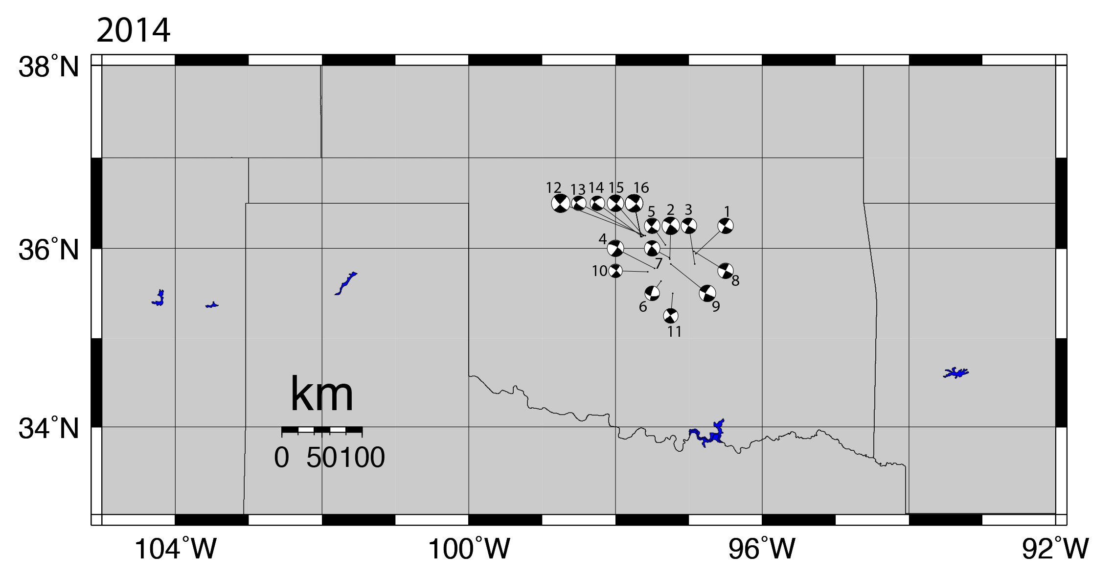
Figure 2. Beach ball diagrams of 16 of the largest earthquakes in Oklahoma in 2014, all showing similar focal mechanisms, which is indicative of induced seismicity.
Earthquake faults don’t all point in the same direction, which means different forces will affect faults differently. Depending on their orientation, some faults might shift in a north-south direction, some might shift in an east-west direction, some might be tilted at an angle, while others are more upright, etc. Seismologists use focal mechanisms to describe the movement of a fault during an earthquake, and these focal mechanisms are depicted by beach ball diagrams (Figure 2). The beach ball diagrams look, literally, like black and white beach balls. Different quadrants of the “beach ball” will be more dominant depending on what type of fault it was and how it moved (See USGS definition of Focal Mechanisms and the “beach ball” symbol).
When an earthquake is triggered by an injection well, it means that the fluid injected into the ground is essentially the straw that broke the camel’s back. Earthquake theory predicts that the forces from an injection well won’t trigger all faults, but only those that are oriented just right. Since we expect that only certain faults with just the right orientation will get triggered, that means we also expect the earthquakes to have similar focal mechanisms, and thus, similar beach ball diagrams. And that’s exactly what we see in Oklahoma.
Cross-correlation programs and beach ball diagrams are only two tools we used at the VTSO to confirm which earthquakes were induced, but seismologists have many means of determining if an earthquake is induced or natural.
Limitations of science?
With so much strong scientific evidence, why can people in industry still claim there isn’t enough science to officially confirm that an injection well triggered an earthquake? In some cases, these claims are simply wrong. In other cases, though, especially in Oklahoma, the problem is that no one was monitoring the disposal wells and the earthquakes from the start. Well operators were not required to publicly track the volumes of water they injected into wells until recently, and no one monitored for nearby earthquake activity. The big problem is not a lack of scientific evidence, but a lack of data from industry to perform sufficient research. Scientists need information about the history, volume, and pressure of fluid injection at a disposal well if they’re to confirm whether or not earthquakes are triggered by it. Often, that information is proprietary and not publically available, or it may not exist at all.
At this point though, two other factors make direct correlations between injection wells and earthquakes in Oklahoma even more difficult:
So many wells have injected signficiant volumes of water in close enough proximity that pointing a finger at a specific well is more challenging.
A large number of wells have injected water for so many years, that the earthquakes are migrating farther and farther from their original source. Again, pointing a finger at a specific well gets harder with time.
What we know
We know what induced seismicity is and why it occurs. We know that if a wastewater injection well disposes of large volumes of fluids deep underground in a region that has existing faults, it will likely trigger earthquakes. We know that if a region previously had few earthquakes, and then sees an uptick in earthquakes after wastewater injection begins, the earthquakes are likely induced. We know that if we want to understand the situation better, we need more seismic stations near disposal wells so we can more accurately monitor the area for seismicity both before and after the well becomes active.
What don’t we know?
We don’t know how big an induced earthquake can get. Oklahoma’s largest earthquake, which was also the largest induced earthquake ever recorded in the United States, was a magnitude 5.6. That’s big enough to cause millions of dollars of damage. Worldwide, the largest earthquake suspected to be induced occurred near the Koyna Dam in India, where a magnitude 6.3 earthquake killed nearly 200 people in 1967.
Can an earthquake that large occur in the central U.S.? The best guess right now: yes.
Seismologists suspect that an induced earthquake could get as big as the size of the fault. If a fault is big enough to trigger a magnitude 7 or 8 earthquake, then that is potentially how large an induced earthquake could be. In the early 1800s, three earthquakes between magnitudes 7 and 8 struck along the New Madrid Fault Zone near St. Louis, Missouri. Toward the end of the 1800s, a magnitude 7 earthquake shook Charleston, South Carolina. In those two areas, injection wells could potentially trigger very large earthquakes.
We have no historic record of earthquakes that large in Oklahoma, so right now, the best guess is that the largest an earthquake could get there would be between a magnitude 6 and 6.5. That would be big enough to cause significant damage, injuries, and possibly death.
The solution
What’s the take-home message from all of this?
First, the science exists to back up the conclusion that wastewater injection wells trigger earthquakes.
Second, if we want to get a better feel for which wells are more problematic, we need funding, seismic stations, and staff to monitor seismic activity around all high-volume injection wells, along with a history of injection times, volumes and pressures at the well.
Third, this is a problem that, if left unchecked, has the potential to result in major damage, incredible expense, and possibly loss of life.
Induced earthquakes are a real phenomenon. While more research is necessary to help us better understand the intricacies of these events and to identify correlations in complex cases, the general cause of the earthquake swarms in Oklahoma and other states is not a mystery. They are man-made problems, backed up by decades of scientific research. They have the potential to create significant damage, but we have the wherewithal to prevent them. We don’t need to go to the extreme of shutting down all wells, but rather, we just need to be able to monitor the wells and ensure that they don’t trigger earthquakes. If a well does trigger an earthquake, then at that point, the well operators can either experiment with significantly decreasing the volume of water that’s injected, or the well can be shut down completely. Understanding and acknowledging the connection between injection wells and earthquakes will make induced seismicity a much easier problem to solve.
The US Food, Energy, Water Interface Examined By Ted Auch, Great Lakes Program Coordinator
With the emergence of concerns about the Food, Energy, Water (FEW) intersection as it relates to oil and gas (O&G) expansion, we thought it was time to dig into the numbers and ask some very simple questions about organic farms near drilling. Below is an analysis of the location and quantity of organic farms with heavy drilling activity in Ohio and nationally. Organic farms rely heavily on the inherent/historical quality of their soils and water, so we wanted to understand whether and how these businesses closest to O&G drilling are being affected.
Key Findings:
Currently 11% of US organic farms are within US O&G Regions of Concern (ROC). However, this number has the potential to balloon to 15-31% if our respective shale plays and basins are exploitated, either partially or in full,
68-74% of these farms produce crops in states like California, Ohio, Michigan, Pennsylvania, and Texas,
Issues such as soil quality, watershed resilience, and water rights are likely to worsen over time with additional drilling.
Methods
To answer this broad question, we divided organic farms in the United States into three categories, depending on whether they were within the:
Core (O&G Wells < 1 mile from each other),
Intermediate (1-3 miles between O&G Wells), or
Periphery (3-5 miles between O&G Wells) of current activity or Regions of Concern (ROC).1
Additionally, from our experience looking at O&G water withdrawal stresses within the largely agrarian Muskingum River Watershed in OH we decided to add to the ROCs. To this end we worked to identify which sub-watersheds (5-10 miles between O&G Wells) and watersheds (10-20 miles between O&G Wells) might be affected by O&G development.
Together, distance from wells and density of development within particular watersheds make up the 5 Regions of Concern (ROCs) (Table 1).
Table 1. Five ROCs under this investigation and what they look like from a mapping perspective
Label
Distance Between Wells
Mapping Visual
Core
< 1 mi
Intermediate
1-3 mi
Periphery
3-5 mi
Sub-Watershed
5-10 mi
Watershed
10-20 mi
We generated a dataset of 19,515 US organic farms from the USDA National Organic Program (NOP) by using the Geocode Address function in ArcGIS 10.2, which resulted in a 100% match for all farms.2
We also extracted soil order polygons within the above 5 ROCs using the NRCS’ STATSGO Derived Soil Order3 dataset made available to us by Sharon Whitmoyer at the USDA-NRCS-NSSC-Geospatial Research Unit and West Virginia University. For those not familiar with soil classification, soil orders are analogous to the kingdom level within the hierarchy of biological classification. Although, in the case of soils there are 12 soil orders compared to the 6 kingdoms of biology.
The National Organic Farms Map
This map shows organic farms across the U.S. that are located within the aforementioned ROCs. Data include certifying agent, whether or not the farm produces livestock, crops, or wild crops along with contact information, farm name, physical address, and specific products produced. View map fullscreen
National Numbers
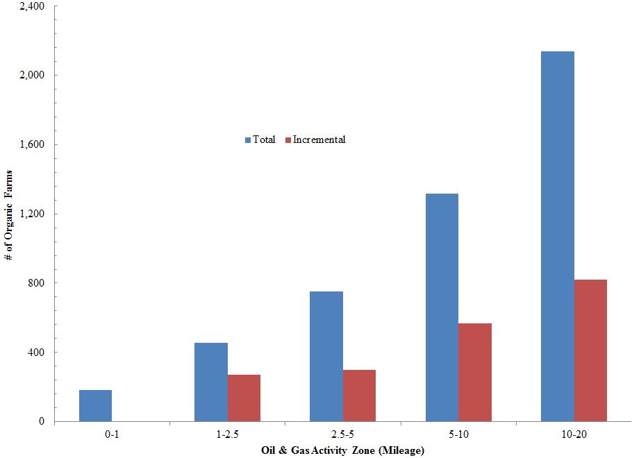
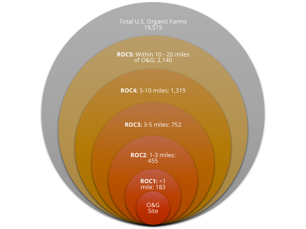
Figure 1. Total and incremental number of US organic farms in the 5 O&G ROCs.
Nationally, the number of organic farms near drilling activity within specific regions of concern are as follows (as shown in Figure 1):
Watershed O&G ROC – 2,140 organic farms (11% of North American organic farms)
Sub-Watershed O&G ROC – 1,319
Periphery O&G ROC – 752
Intermediate O&G ROC – 455
Core O&G ROC – 183
Ohio’s Organic Farms Near Drilling
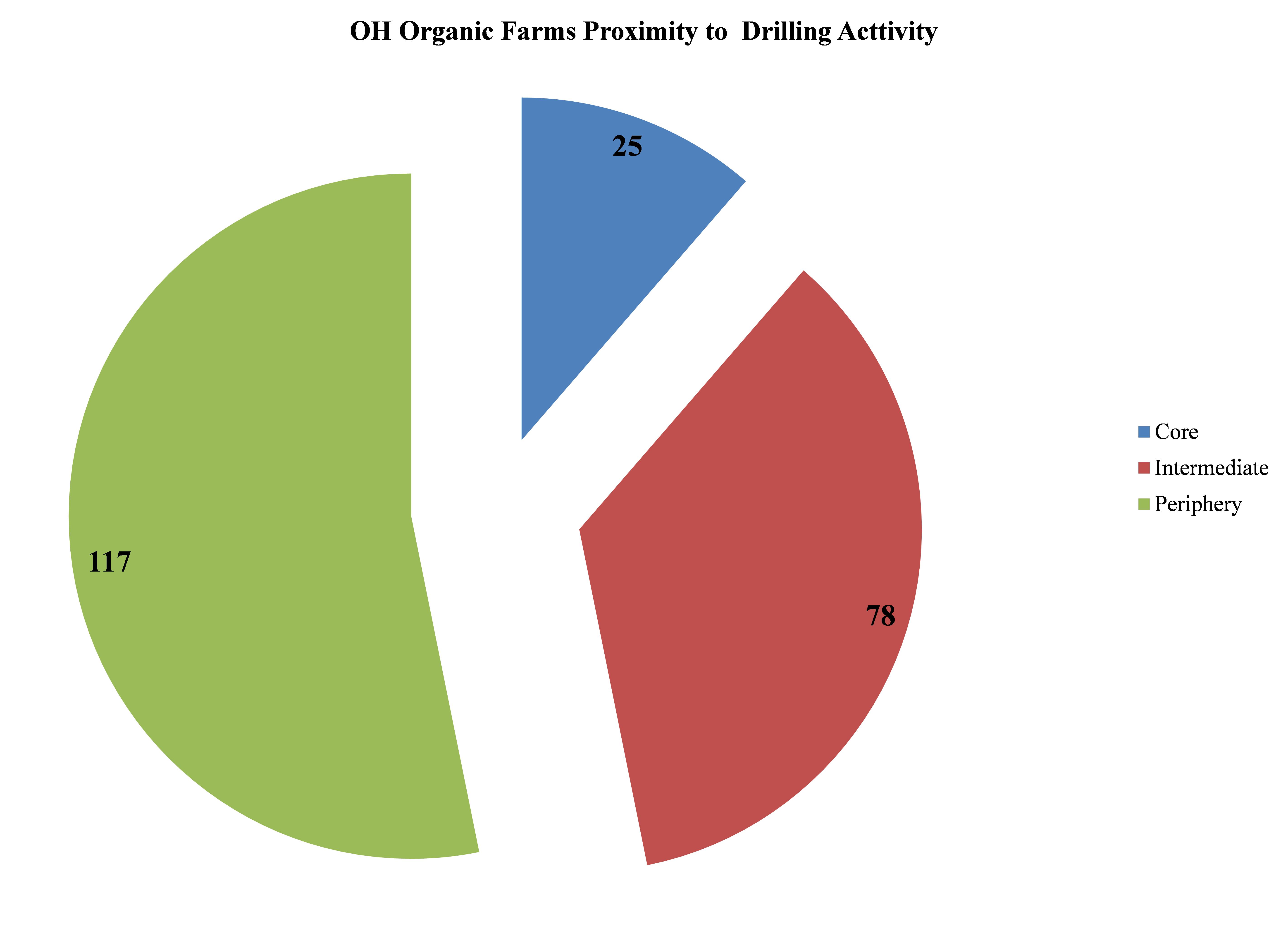
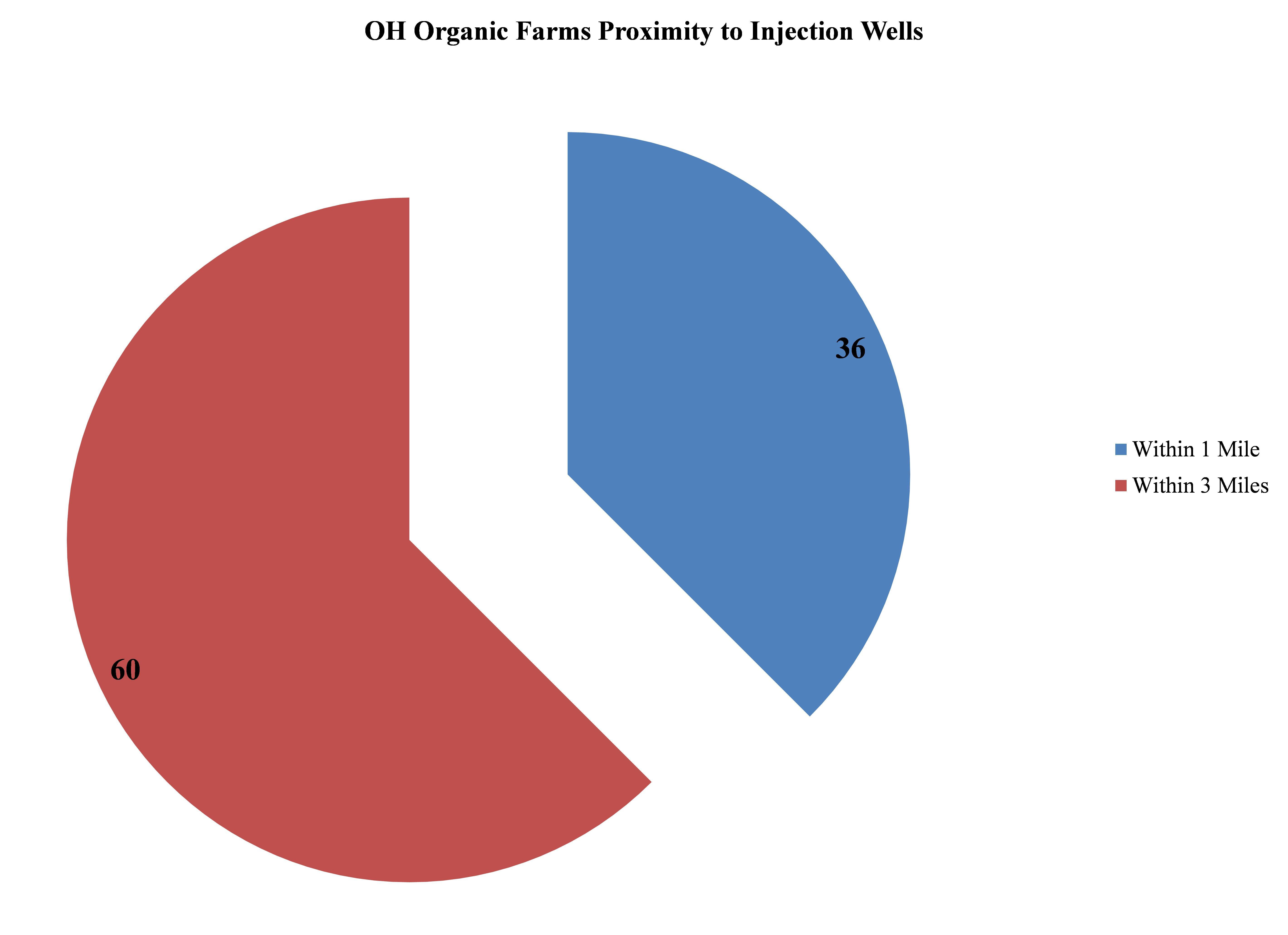
The following key statistics stood out among the analyses for OH’s 703 (3.6% of US total) organic farms. Figures 2 & 3 show how many farms are near drilling activity and injection (disposal) wells in OH. Click the images to view fullsize graphics:
Figure 2. OH Organic Farms Proximity to Drilling Activity
Figure 3. OH Organic Farms Proximity to Injection Wells
Potential Trends
If oil and gas extraction continues along the same path that we have seen to-date, it is reasonable to expect that we could see an increase in the number of organic farms near this industrial activity. A few figures that we have worked up are shown below:
2,912 Organic Farms in the US Shale Plays (15% of total organic farms)
Another way to look at these five ROCs when asking how shale gas build-out will interact with and/or influence organic farming is to look at the soils beneath these ROCs. What types of activity do they currently support? The productivity of organic farms, as well as their ability to be labeled “organic,” are reliant upon the health of their soils even more so than conventional farms. Organic farms cannot rely on synthetic fertilizers, pesticides, herbicides, or related soil amendments to increase productivity. Soil manipulation is prohibitive from a cost and options perspective. Thus, knowing what types of soils the shale industry has used and is moving towards is critical to understanding how the FEW dynamic will play out in the long-term. There is no more important variable to the organic farmer sans freshwater than soil quality and diversity.
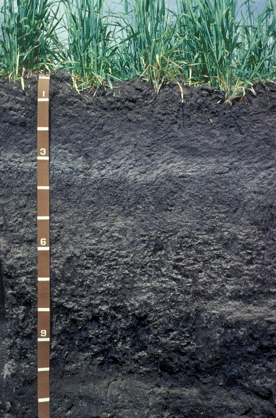
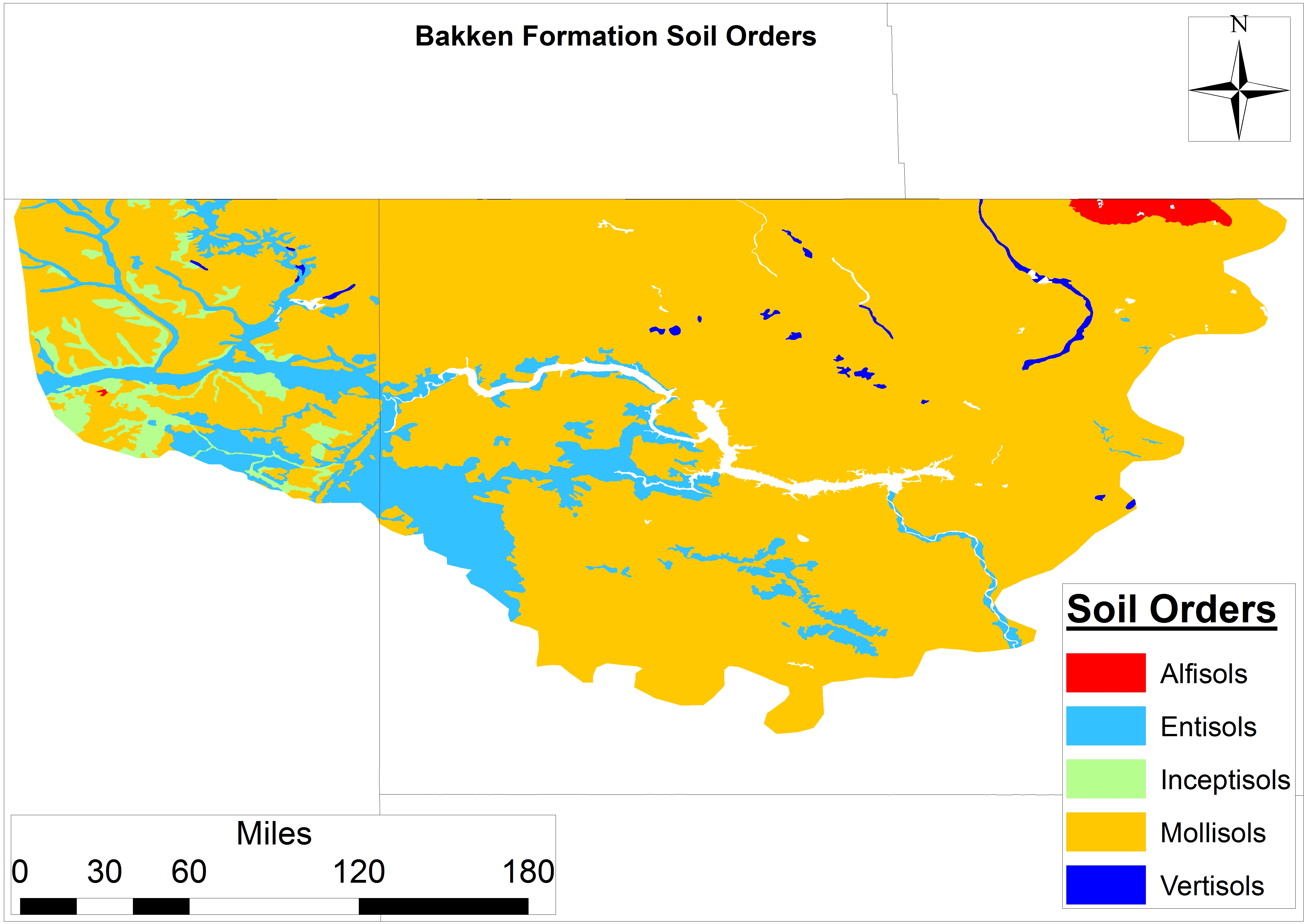
The soils of most concern under this analysis are the Prairie-Forest Transition soils of the Great Lakes and Plains, commonly referred to as Alfisols, and the Carbon-Rich Grasslands or Mollisols (Figure 4 & 5). The latter is proposed by some as a soil order worthy of protection given our historical reliance on its exceptional soil fertility and support for the once ubiquitous Tall Grass Prairies. Both soils face a second potential wave of O&G development, with a combined 18,660 square miles having come under the influence of the O&G industry within the Core ROC and an additional 58-108,000 square miles in the Intermediate and Periphery ROCs. If the watersheds within these soils and O&G co-habitat were to come under development, total potential Alfisol and Mollisol alteration could reach 273,200 square miles. This collection of soils currently accounts for 43-47% of the Core and Intermediate O&G ROCs and would “stabilize” at 50-51% of O&G development if the watersheds they reside in were to see significant O&G exploration.
Figure 6. The five soil orders within the Bakken Shale formation in Montana and North Dakota.
These same soils sit beneath or have been cleared for much of our wheat, corn, and soybean fields – not to mention much of the Bakken Shale exploration to date (Figure 6, above)
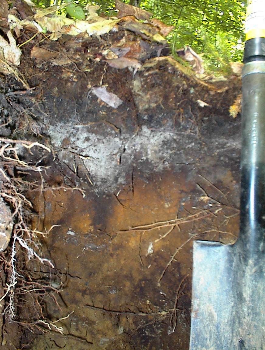
The three forest soil orders (i.e., Spodosol, Ultisol, and Andisol shown in Figures 7-9) account for 9,680-20,529 square miles of the Core and Intermediate O&G ROCs, which is 22 and 17% of those ROC’s, respectively. If we assume future exploration into the Periphery and Watershed ROC we see that forest soils will become less of a concern, dropping to 14-15% of these outlying potential plays, with the same being true for the two Miscellaneous soil types. The latter will decline from 28% to 25% of potential O&G ROCs.
Figure 7. Ultisol – Courtesy of the University of Georgia
Figure 8. Spodosol – Courtesy of the Hubbard Brook Experimental Forest
Figure 9. Andisol – Courtesy of USDA’s NRCS
Figure 10. Histosol, – Courtesy of Michigan State University
If peripheral exploration were to be realized, another soil type will have to fill this gap. Our analysis demonstrates this gap would be filled by either Organic Wetlands or Histosols, which currently constitute <200 and 529 square miles of the Core and Intermediate ROCs, respectively (Figure 10). For so many reasons wetland soils are crucial to the maintenance and enhancement of ecosystem services, wildlife migration, agricultural productivity, and the capture and storage of greenhouse gases. However, if O&G exploration does expand to the Periphery ROC and beyond we would see reliance on wetland soils increase nearly 15 fold (i.e., 16% of Lower 48 wetland soil acreage).
The quality of these wetlands is certainly up for debate. However, what is fact is that these wetlands would be altered beyond even the best reclamation techniques. We know from the reclamation literature that the myriad difficulties associated with reassembling prior plant wetland communities. Finally, it is worth noting that a similar uptick in O&G reliance on arid (i.e., extremely unproductive but unstable) soils is may occur with future industry expansion. These soils will, as a percent of all ROCs, increase from 7% to 9% (i.e. 10-11% of all lower 48 arid soil acreage).
What do these changes mean for the agriculture industry in OH?
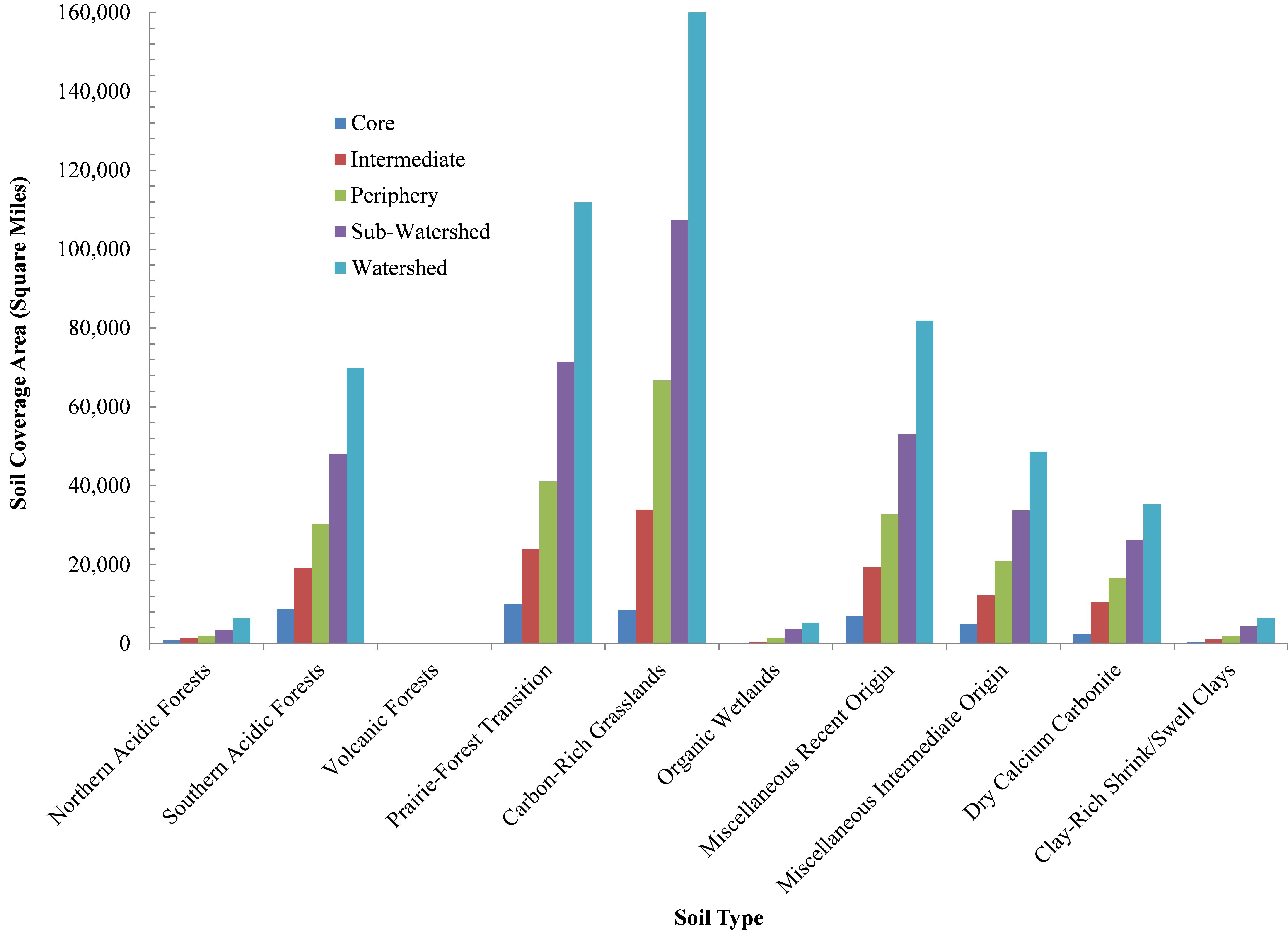
If these future O&G exploration scenarios were to play out, we estimate 20-22% of Southern Acidic Forest, Prairie-Forest Transition, Miscellaneous Recent Origin, and Carbon-Rich Grassland soils will have been effected or dramatically altered due to O&G land-use/land-cover (LULC) change nationally (Figure 11). This decline in productivity is likely familiar to communities currently grappling with how to manage a dramatically different landscape post-shale introduction in counties like Bradford in PA and Carroll in OH. The effects that such alteration has had and will have on landscape productivity, wildlife habitat fragmentation, and hydrological cycles is unknown but worthy of significant inquiry.
These questions are important enough to have received a session at Ohio Ecological Food and Farming Association’s (OEFFA) 2015 conference in Granville last month and were deemed worthy of a significant grant to The FracTracker Alliance from the Hoover Foundation aimed at quantifying the total LULC footprint of the shale gas industry across three agrarian OH counties. Early results indicate that every acre of well-pad requires 5.3 acres of gathering lines along with nearly 14 miles of buried pipelines – most of which are beneath high quality wetlands. This study speaks to the potential for 20-30% of the state’s Core Utica Region – or 10-15% of the Expanded Utica Region4 – being altered by shale gas activity.
Figure 11. National distribution of soil types within the 5 ROCs under consideration: 1) Forest Soils, 2) Prairie/Agriculture soils, 3) Organic Wetlands, 4) Miscellaneous soils, 5) Dry Soils.
Figure 11 Description:
Forest Soils – Northern and Southern Acidic Forests, Volcanic Forests,
Prairie/Agriculture – Prairie-Forest Transition and Carbon-Rich Grasslands,
Organic Wetlands
Miscellaneous – Recent and Intermediate Origins,
Dry Soils – Dry Calcium Carbonite and Clay-Rich Shrink/Swell Clays
Conclusion
The current and potential interaction(s) between the O&G and organic farming industries is nontrivial. Currently 11% of US organic farms are within what we are calling O&G ROCs. However, this number has the potential to balloon to 15-31% if our respective shale plays and basins are exploited, either partially or in full. Most of these (68-74%) are crop producers in states like California, Ohio, Michigan, Pennsylvania, and Texas.
Issues such as soil quality – specifically Prairie-Forest, Carbon Rich Grasslands, and Wetland soils – watershed resilience, and water rights are likely to become of more acute regional concern as the FEW interactions become increasingly coupled. How and when this will play out is anyone’s guess, but its play out is indisputable. Agriculture is going to face many staunch challenges in the coming years, as the National Science Foundation5 wrote:
The security of the global food supply is under ever-increasing stress due to rises in both human population and standards of living world-wide. By the end of this century, the world’s population is expected to exceed 10 billion, about 30% higher than today. Further, as standards of living increase globally, the demand for meat is increasing, which places more demand on agricultural resources than production of vegetables or grains. Growing energy use, which is connected to water availability and climate change, places additional stress on agriculture. It is clear that scientific and technological breakthroughs are needed to produce food more efficiently from “farm to fork” to meet the challenge of ensuring a secure, affordable food supply.
An additional 69 organic farms were geo-referenced in Canada and 7,524 across the globe for a similar global analysis to come.
Description of STATSGO2 Database and associated metadata here.
Core Utica Regions include any county that has ≥10 Utica permits to date and Expanded Utica Region includes any county that has 1 or more Utica permits.
By the Mathematical and Physical Sciences Advisory Committee – Subcommittee on Food Systems in “Food, Energy and Water: Transformative Research Opportunities in the Mathematical and Physical Sciences”
https://www.fractracker.org/a5ej20sjfwe/wp-content/uploads/2015/03/OrganicFarms-Feature.jpg400900Ted Auch, PhDhttps://www.fractracker.org/a5ej20sjfwe/wp-content/uploads/2025/09/2025-Wordmark-Logo.pngTed Auch, PhD2015-03-11 15:00:572020-07-21 10:32:10Organic farms near drilling activity in the U.S. and Ohio
By Juliana Henao & Samantha Malone, FracTracker Alliance
Currently, 11% (2,140 of 19,515 total) of all U.S. organic farms share a watershed with active O&G drilling. Additionally, this percentage could rise up to 31% if unconventional O&G drilling continues to grow.
Organic farms represent something pure for citizens around the world. They produce food that gives people more certainty about consuming chemical-free nutrients in a culture that is so accustomed to using pesticides, fertilizers, and herbicides in order to keep up with booming demand. Among their many benefits, organic farms produce food that is high in nutritional value, use less water, replenish soil fertility, and do not use pesticides or other toxic chemicals that may get into our food supply. To maintain their integrity, however, organic farms have an array of regulations and an extensive accreditation process.
What does it mean to be an organic farm?
The accreditation process for an organic farm is quite extensive. USDA organic regulations include:
The producer must manage plant and animal materials to maintain or improve soil organic matter content in a manner that does not contribute to contamination of crops, soil, or water by plant nutrients, pathogenic organisms, heavy metals, or residues of prohibited substance.
No prohibited substances can be applied to the farm for a period of 3 years immediately preceding harvest of a crop
The farm must have distinct, defined boundaries and buffer zones, such as runoff diversions to prevent the unintended application of a prohibited substance to the crop or contact with a prohibited substance applied by adjoining land that is not under organic management.
There are additional regulations that pertain to crop pest, weed, and disease standards; soil fertility and crop nutrient management standards; seeds and planting stock practice standards; and wild-crop harvesting practice standards, to name a few. A violation of any one of these USDA regulations can mean a hold on the accreditation of an organic farm.
The full list of regulations and requirements can be found here.
Threats Posed by Oil & Gas
Nearby oil and gas drilling is one of many threats to organic farms and their crop integrity. With a steady expansion of wells, the O&G industry is using more and more land, requiring significant quantities of fresh water, and emitting air and water pollution from sites (both in permitted and unpermitted cases). O&G activity could not only affect the quality of the produce from these farms, but also their ability to meet the USDA’s organic standards.
To see how organic farms and the businesses surrounding wells are being affected, Ted Auch analyzed certain dynamics of organic farms near drilling activity in the United States, and generated some key findings. His results showcase how many organic farms are at risk now and in the future if O&G drilling expands. Below we describe a few of his key findings, but you can also read the entire article here.
Key Findings – Organic Farms Near Oil & Gas Activity
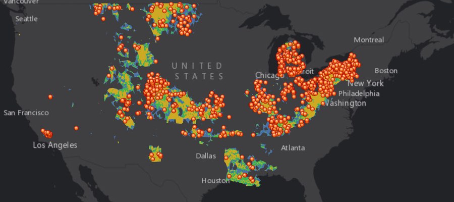
Explore this dynamic map of the U.S. organic farms (2,140) within 20 miles of oil & gas drilling. To view the legend and see the map fullscreen, click here.
Of the 19,515 U.S. organic farms in the U.S., 2,140 (11%) share a watershed with oil and gas activity – with up to 31% in the path of future wells in shale areas. Why look at oil and gas activity at the watershed level? Watersheds are key areas from which O&G companies pull their resources or into which they emit pollution. For unconventional drilling, hydraulic fracturing companies need to obtain fresh water from somewhere in order to frack the wells, and often the local watershed serves as that source. Spills can and do occur on site and in the process of transporting the well pad’s products, posing risks to soils and waterways, as well.
Figure 1, below, demonstrates the number of organic farms near active oil & gas wells in the U.S. – broken down by five location-based Regions of Concern (ROC).
Figure 1: Total and incremental numbers of US organic farms in the 5 O&G Regions of Concern (ROC).
The most at-risk farms are located in five states: California, Ohio, Michigan, Texas and Pennsylvania. Learn more about the breakdown of the types of organic farms that fall within these ROCs, including what they produce.
Out of Ohio’s 703 organic farms, 220 organic farms are near drilling activity, and 105 are near injection (waste disposal) wells.
Conclusion
More and more O&G drilling is being permitted to operate near organic farms in the United States. The ability for municipalities to zone out O&G varies by state, but there is currently no national restriction that specifically protects organic farms from this industrial activity. As the O&G industry expands and continues to operate at such close proximities to organic farms in the US, there are a variety of potential impacts that we could see in the near future. The following list and more is explained in further detail in Auch’s research paper:
A complete alteration in soil composition and quality,
A need to restore wetland soils that are altered beyond the best reclamation techniques,
A dramatic decline in organic farm and land productivity,
https://www.fractracker.org/a5ej20sjfwe/wp-content/uploads/2015/03/Farm-Rig-Feature.jpg400900FracTracker Alliancehttps://www.fractracker.org/a5ej20sjfwe/wp-content/uploads/2025/09/2025-Wordmark-Logo.pngFracTracker Alliance2015-03-11 15:00:132020-07-21 10:32:1011% of organic farms near drilling in US, potentially 31% in future
By Ted Auch, Great Lakes Program Coordinator, FracTracker Alliance
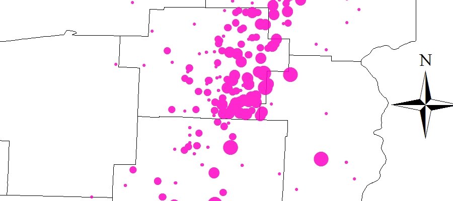
We know from the most recent Ohio Department of Natural Resources (ODNR) permitting numbers that Carroll County, Ohio is home to 26% (461 of 1,778) of the state’s Utica permits and 43% (312 of 712) of all producing wells as of the end of Q3-20141 (Figure 1). But does that mean that the county will continue to see that kind of industrial activity for the foreseeable future? The primary question we wanted to ask with this latest piece is whether the putative “king” of the state’s Utica shale gas counties is indeed Carroll County.
Fig 1. Ohio’s Utica Permits within & adjacent to the Muskingum River Watershed as of February, 2015
To do this we compiled an inventory of annual (2011-2012) and quarterly OH shale gas production numbers for 721 laterals throughout southeast OH.
Permitting and production numbers are not necessarily part and parcel to determine if Carrol Co is truly the king. We decided to investigate the production data and do a simple compare and contrast with the rest of the state’s 409 laterals on one side (ROS) and the 312 Carroll laterals on the other – focusing primarily on days of production and resulting oil, gas, and brine (Table 1 and infographic below).
Carroll vs. ROS Results
Permitting Numbers Breakdown
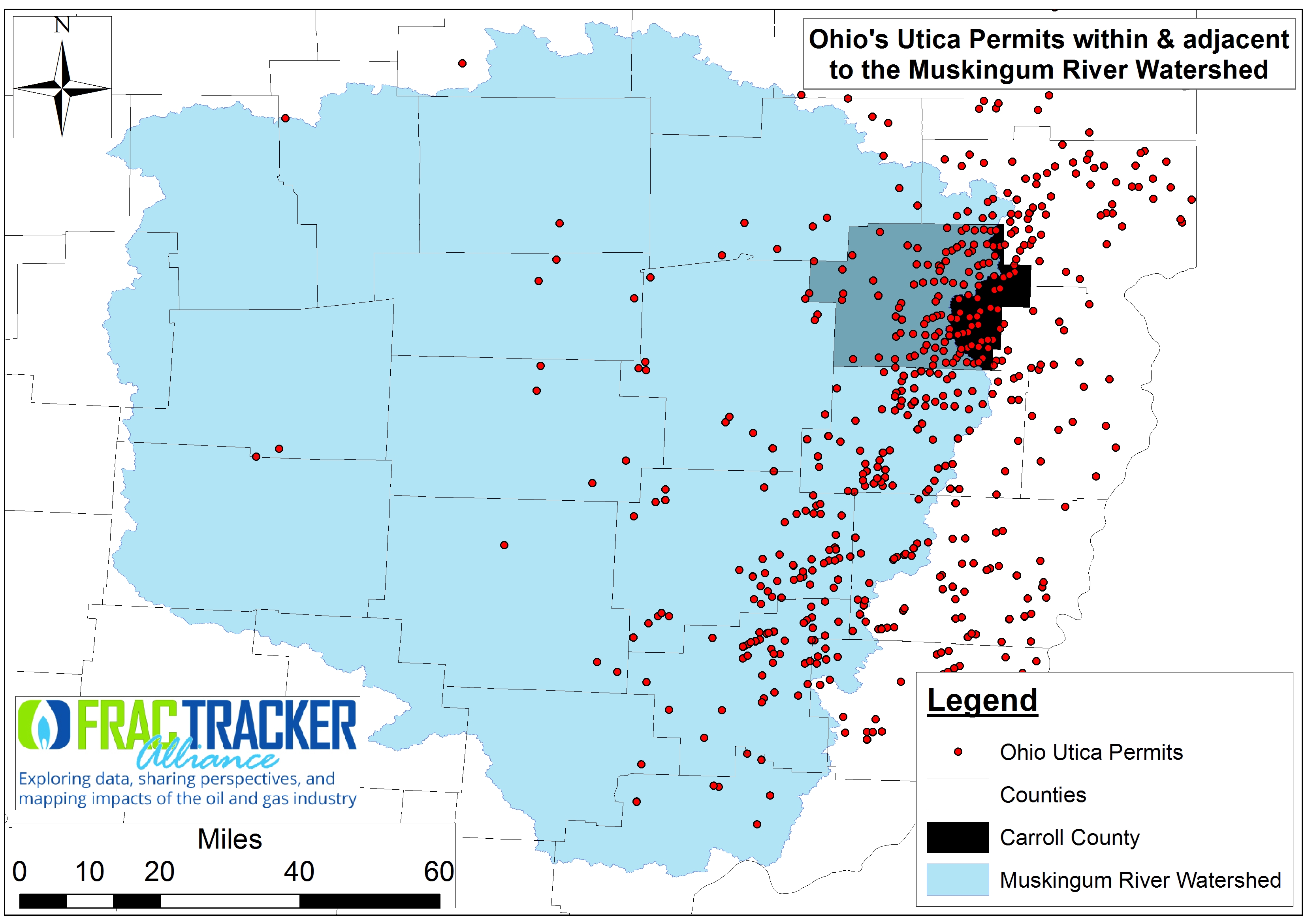
Fig 2. Monthly & cumulative Utica Shale permitting activity in Carrol County, OH vs. the ROS between September 2010 & January 2015
Between the initial permitting phase of September 2010 and January 2105 the number of Utica Shale permits issued in the ROS has averaged 29 per month vs. 10 per month in Carroll County. Permitting actually increased twofold in the ROS in the last 12 months (Figure 2). Conversely, permitting in Carroll County seems to have reached some sort of a steady state, with monthly permitting declining by 23% in the last 12 months. Carroll’s Utica permits generally constituted 47% of all permitting in OH but more recently has dipped to 44%. Newer areas of focus include Belmont, Guernsey, Noble, and Columbiana counties, just to name a few.
Production Days
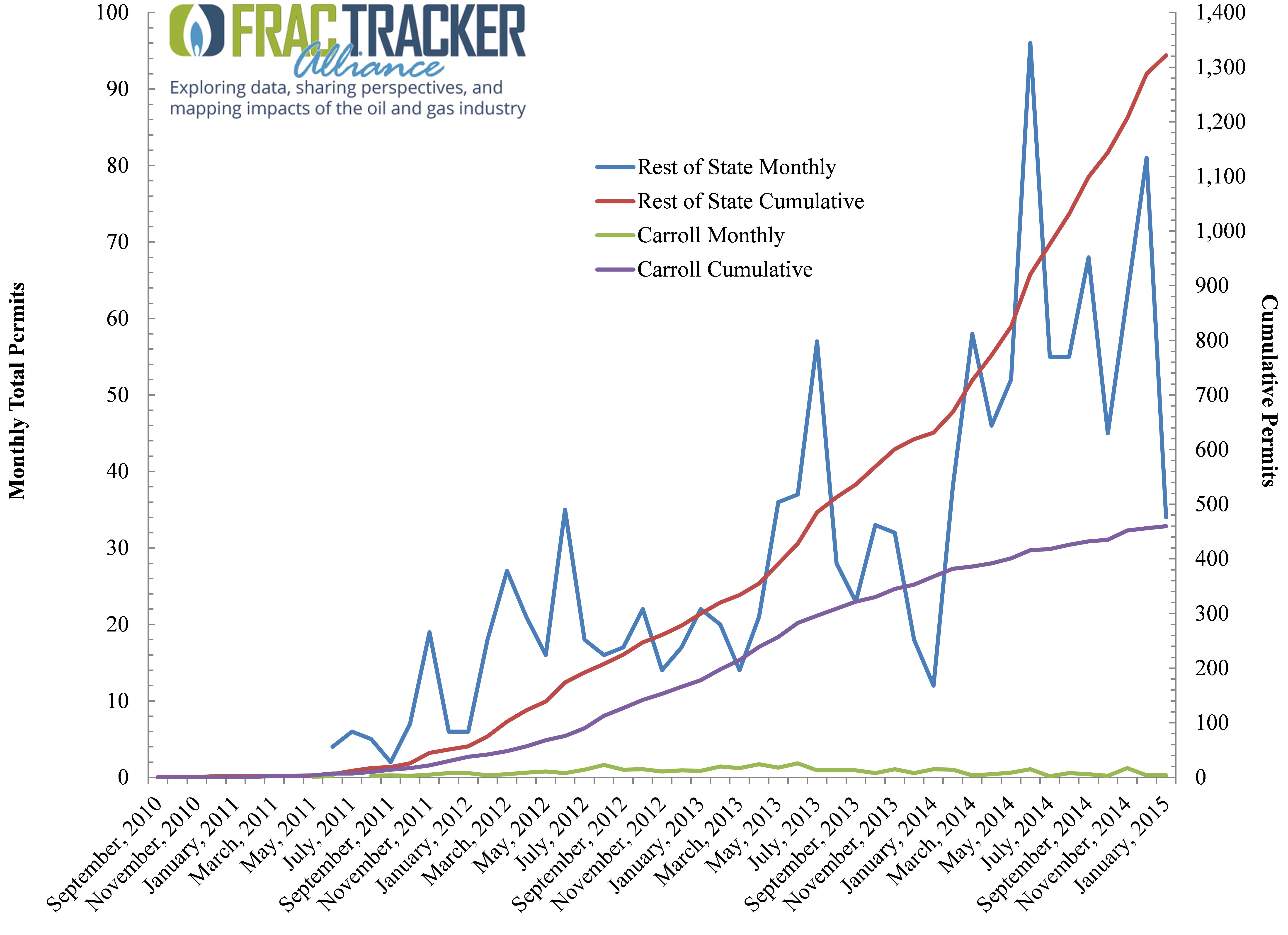
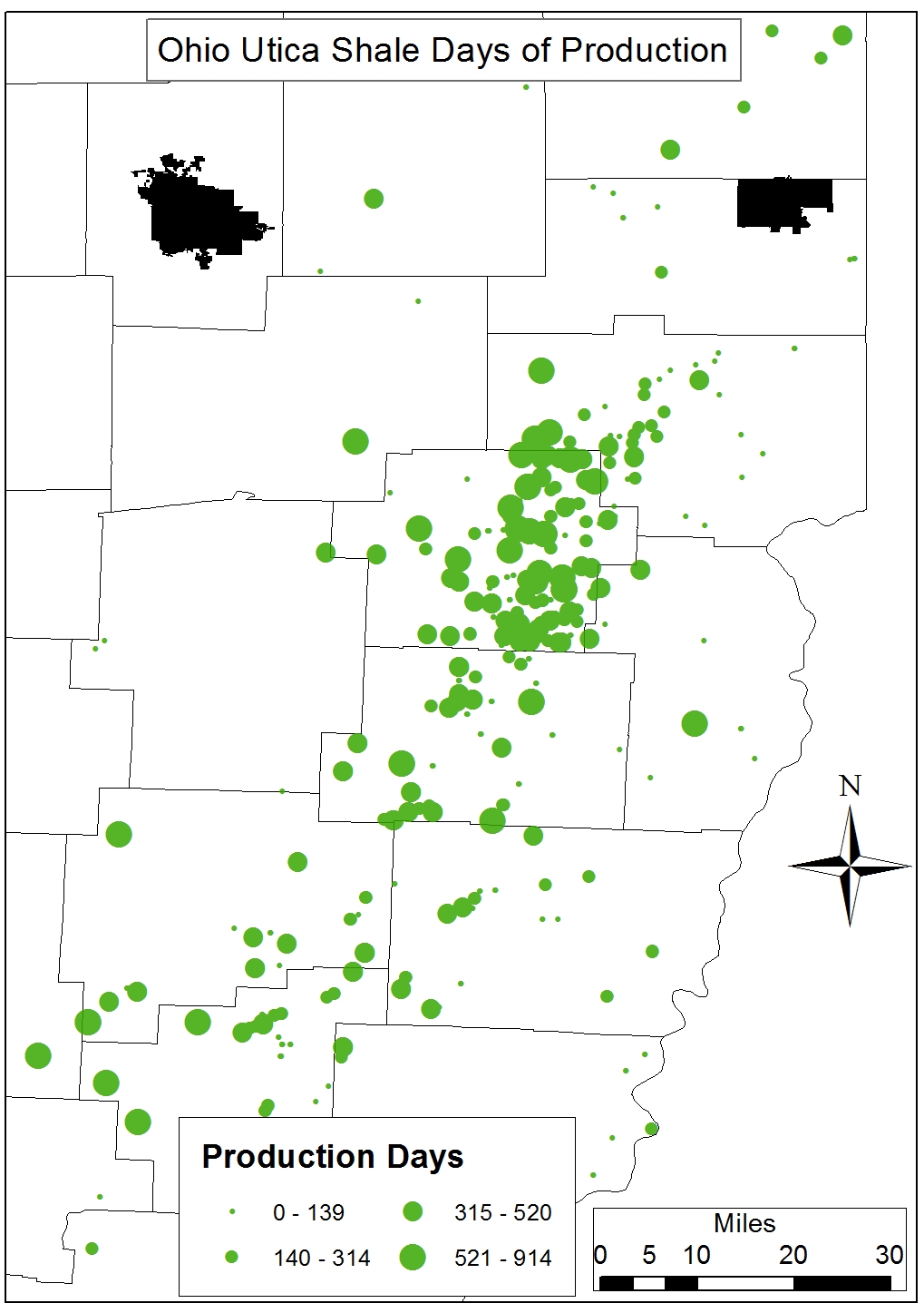
Days in production is a proxy for road activity and labor hours. Carroll’s wells have the rest of the state beat for that metric, with an average of 292 (±188 days) days. The state average is 192 days, with significant well-to-well variability (±177 days). If we assume there was a total of 1,369 possible production days between 2011 and the end of Q3-2014, these averages translate to 21% and 14% of total possible production days for Carroll and ROS, respectively.
Oil Production
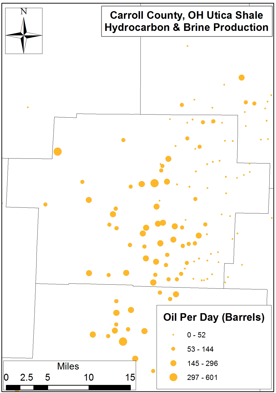
Carroll falls short of the ROS on a total and per-day basis of oil production, although the 442-barrel difference in total oil production is likely not significant. Carroll wells are producing 74 barrels of oil per day (OPD) (±73 OPD) compared to 96 OPD (±122 OPD) for the rest of the state; however, well-to-well variability is so large as to make this type of comparison quite difficult at this juncture. Fifty-seven percent of OH’s 11,361,332 barrels of Utica oil has been produced outside of Carroll County to date. This level of production is equivalent to 16,231 rail tanker cars and roughly 00.18% of US oil production between 2011 and 2013.
This number of rail tanker cars is equivalent to 6% of the US DOT-111 fleet, or 184 miles worth of trains – enough to stretch from Columbus to Pittsburgh.
Natural Gas
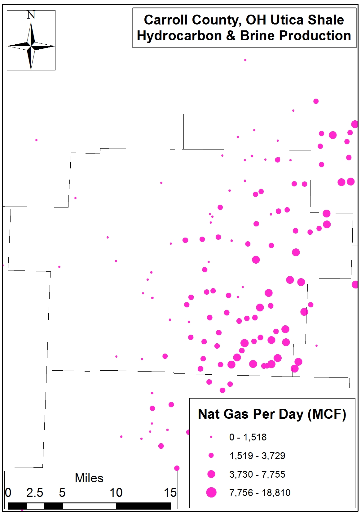
The natural gas story is mixed, with Carroll’s 312 wells having produced 13,430 MCF more than the ROS wells. On a per-well basis, however, the latter are producing 3,327 MCF per day (MCFPD) (±3,477 MCFPD) relative to the 2,155 MCFPD (±1,264 MCFPD) average for Carroll’s wells. Yet again, well-to-well variability – especially in the case of the 409 ROS wells – is high enough that such simple comparisons would require further statistical analysis to determine whether differences are significant or not.
The natural gas produced here in OH currently amounts to roughly 00.51% of U.S. Natural Gas Marketed Production, according to the latest data from the EIA.
Waste – Brine
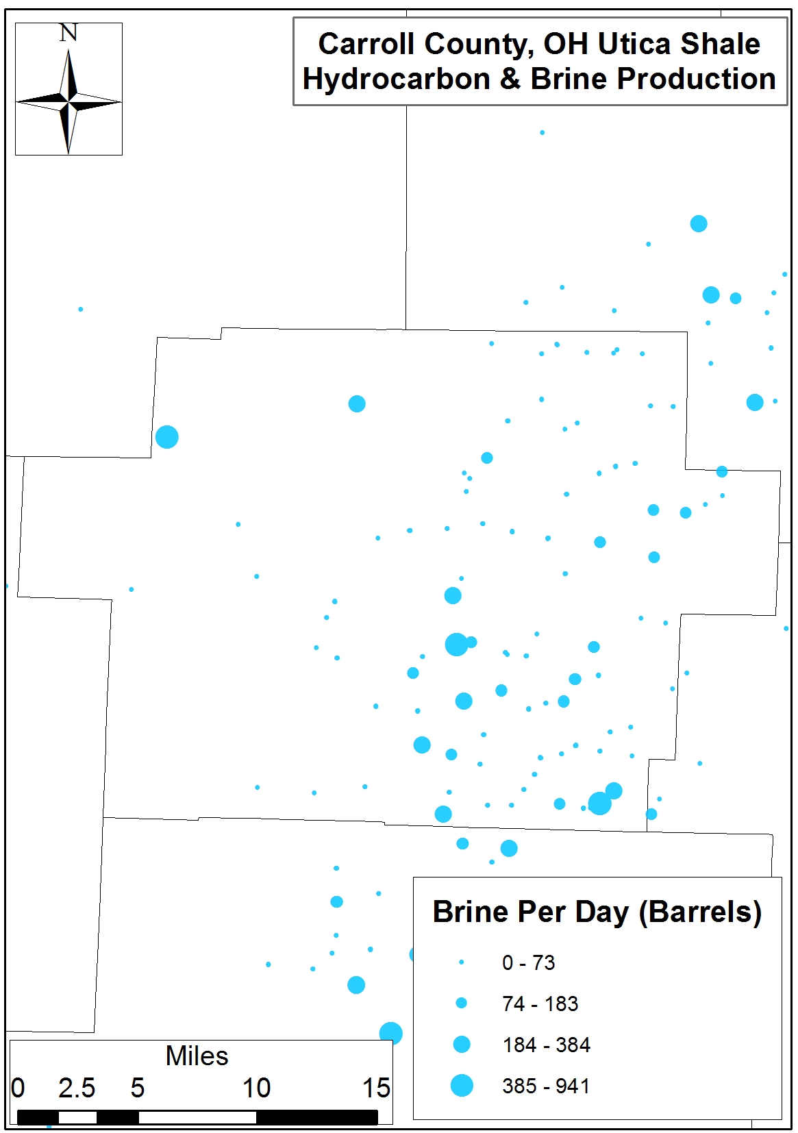
From a waste generation point of view, the ROS laterals have produced 41 more barrels of brine per day (BPD) than the Carroll laterals and 1,465 BPD since production began in 2011. On a per-day basis, the ROS laterals are producing more oil than waste at a rate of 1.92 barrels of oil per barrel of brine waste. Conversely, since production began these respective sums result in Carroll County laterals having produced 1.56 barrels of oil for every barrel of brine vs. the 1.40 oil-to-brine ratio for the ROS. Finally, it is worth noting that the 7,775,130 barrels of brine produced here in OH amounts to 13% of all fracking waste processed by the state’s 235+ Class II Injection wells.
What do these figures mean?
As we begin to compare OH’s Utica Shale expectations vs. reality we see that the “sweet spot” of the play is truly a moving target. The train seems to have already left – or is in the process of leaving – the station in Carroll County (Figures 3 and 4). It seems two of the most important questions to ask now are:
How will this rapidly shifting flow of capital, labor, and resources affect future counties deemed the next best thing? and
What will be left in the wake of such hot money flows?
Answers to these questions will be integral to the preparation for the inevitable sudden or slow-and-steady decline in shale gas activity. These dropouts are just the most recent in a long line of boom-bust cycles to have been foisted on Southeast OH and Appalachia. Effects will include questions regarding watershed resilience, local and regional resource utilization (Figures 5 and 6), social cohesion, tax-base uncertainty, roads, and a rapidly changing physical landscape.
Whether Carroll County can maintain its perch on top of the OH shale mountain is far from certain, but whether it will have to begin to – or should have already – prepare for the downside of this cliff is fact based on the above analysis.
Additional Figures and Charts
Table 1. Carroll County, OH production days and production of oil, gas, and brine on a per-day basis and in total between 2011 and Q3-2014 vis à vis the “Rest of State”
Variable
Carroll (312)
Rest of State (409)
Max
Sum
Mean
Max
Sum
Mean
Total Days
914
91,193
292±188
898
78,430
192±177
Oil (Barrels)
Per Day
453
23,190
74±73
601
39,109
96±122
Total
83,098
4,838,147
15,507
129,005
6,523,185
15,949
Gas (MCF)
Per Day
6,774
672,391
2,155±1,264
18,810
1,360,923
3,327±3,477
Total
2,196,240
168,739,064
540,830
3,181,013
215,706,401
527,400
Brine (Barrels)
Per Day
941
18,516
59±87
810
40,839
100±120
Total
36,917
3,105,260
9,953
99,095
4,669,870
11,418
Oil Per Unit of Brine
Per Day
1.25
1.92
Total
1.56
1.40
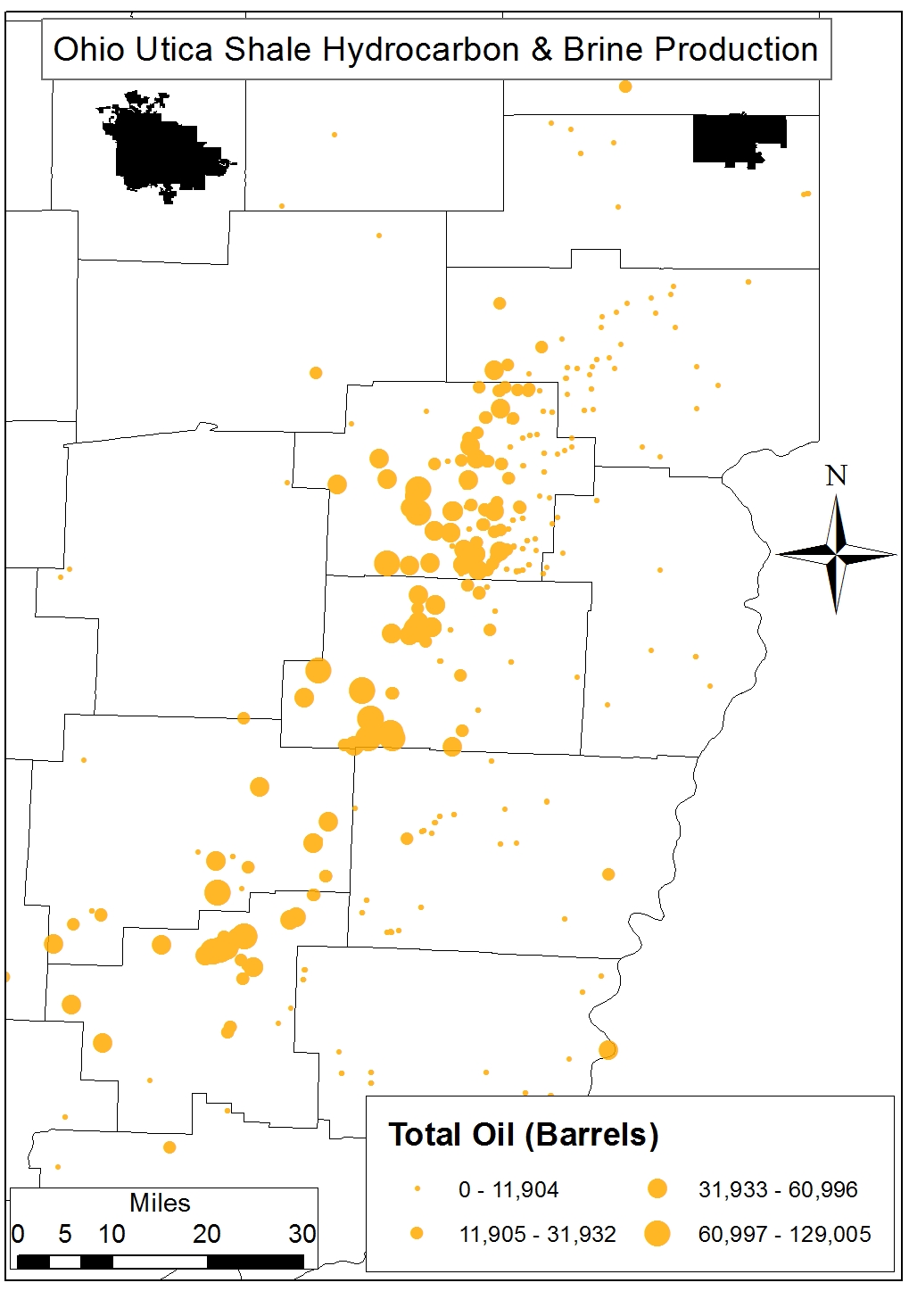
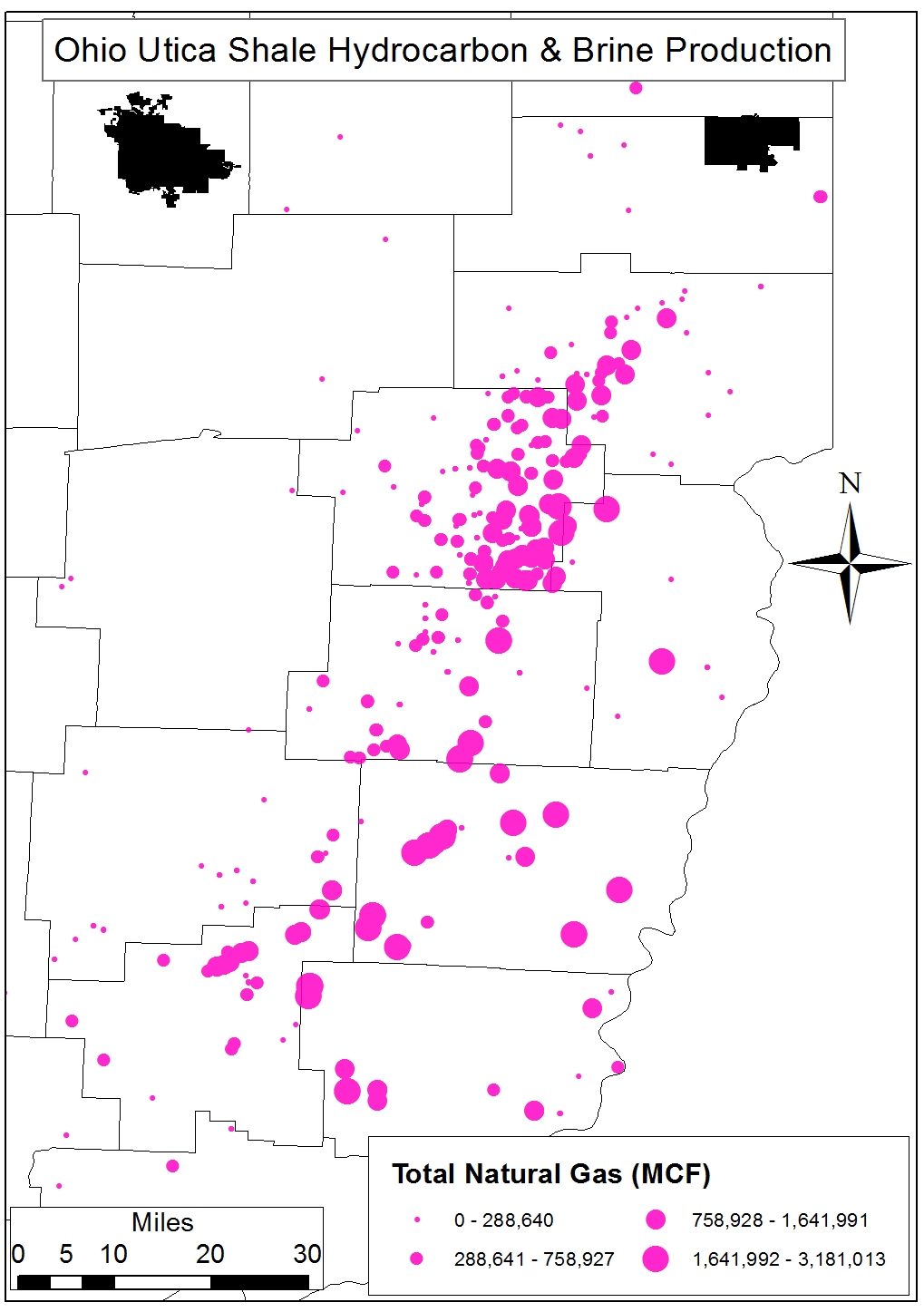
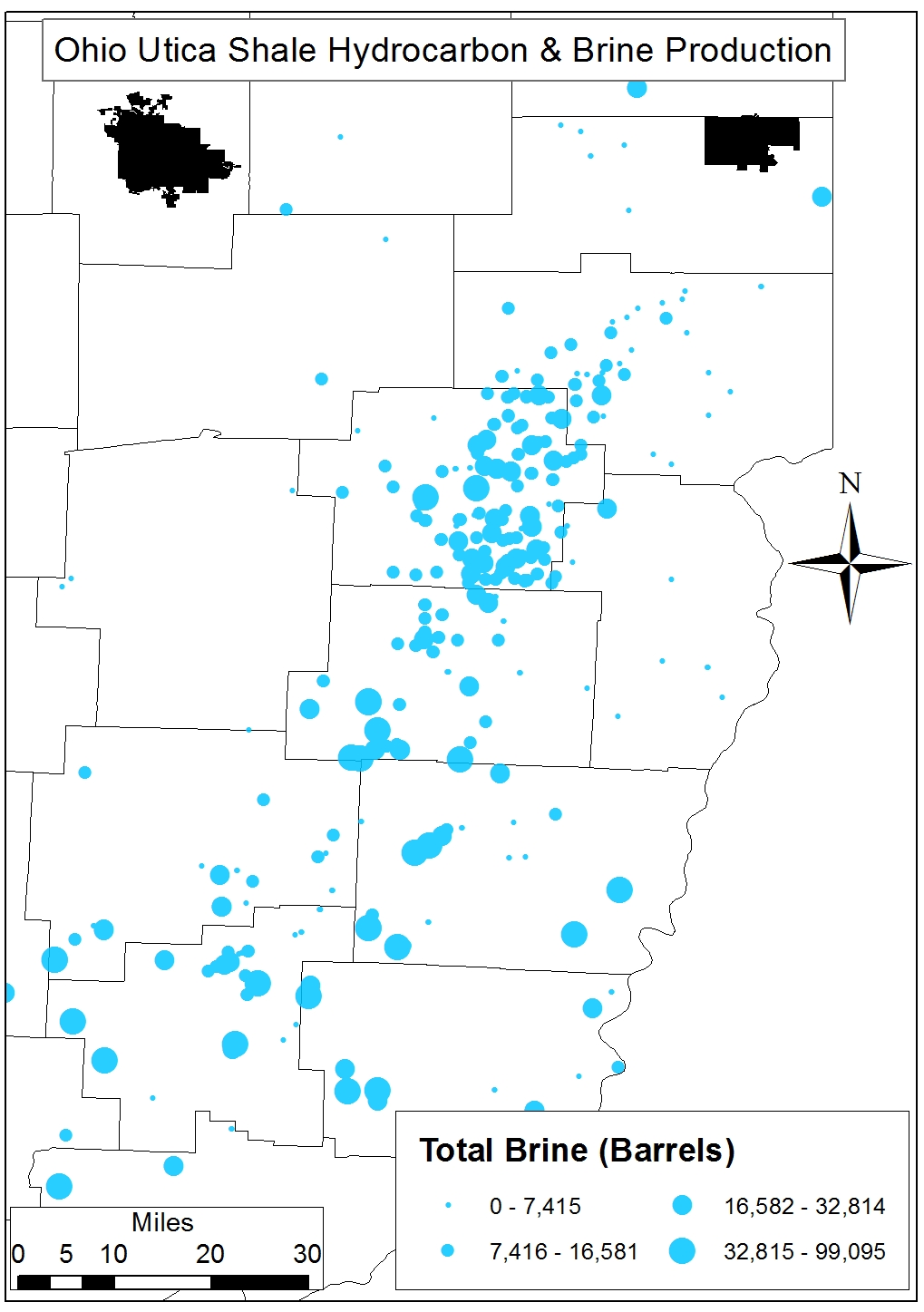
Figures 3a-d. Spatial distribution of Carroll County Utica Shale production days, oil (barrels), natural gas (MCF), and brine (barrels) on a per-day basis.
Fig 3a. Spatial distribution of Carroll Co. Utica Shale production days
Fig 3b. Spatial distribution of Carroll Co. Utica Shale oil (barrels) production on per-day basis
Fig 3c. Spatial distribution of Carroll Co. Utica Shale natural gas (MCF) production on per-day basis
Fig 3d. Spatial distribution of Carroll County Utica Shale brine (barrels) production on a per-day basis
Figures 4a-d. Spatial distribution of OH Utica Shale production days, oil (barrels), natural gas (MCF), and brine (barrels) on a per-day basis.
Fig 4a. Ohio Utica Shale Total Production Days, 2011-2014
Fig 4b. Ohio Utica Shale Total Oil Production (Barrels), 2011-2014
Fig 4c. Ohio Utica Shale Total Natural Gas Production (MCF), 2011-2014
Fig 4d. Ohio Utica Shale Total Brine Production (Barrels), 2011-2014
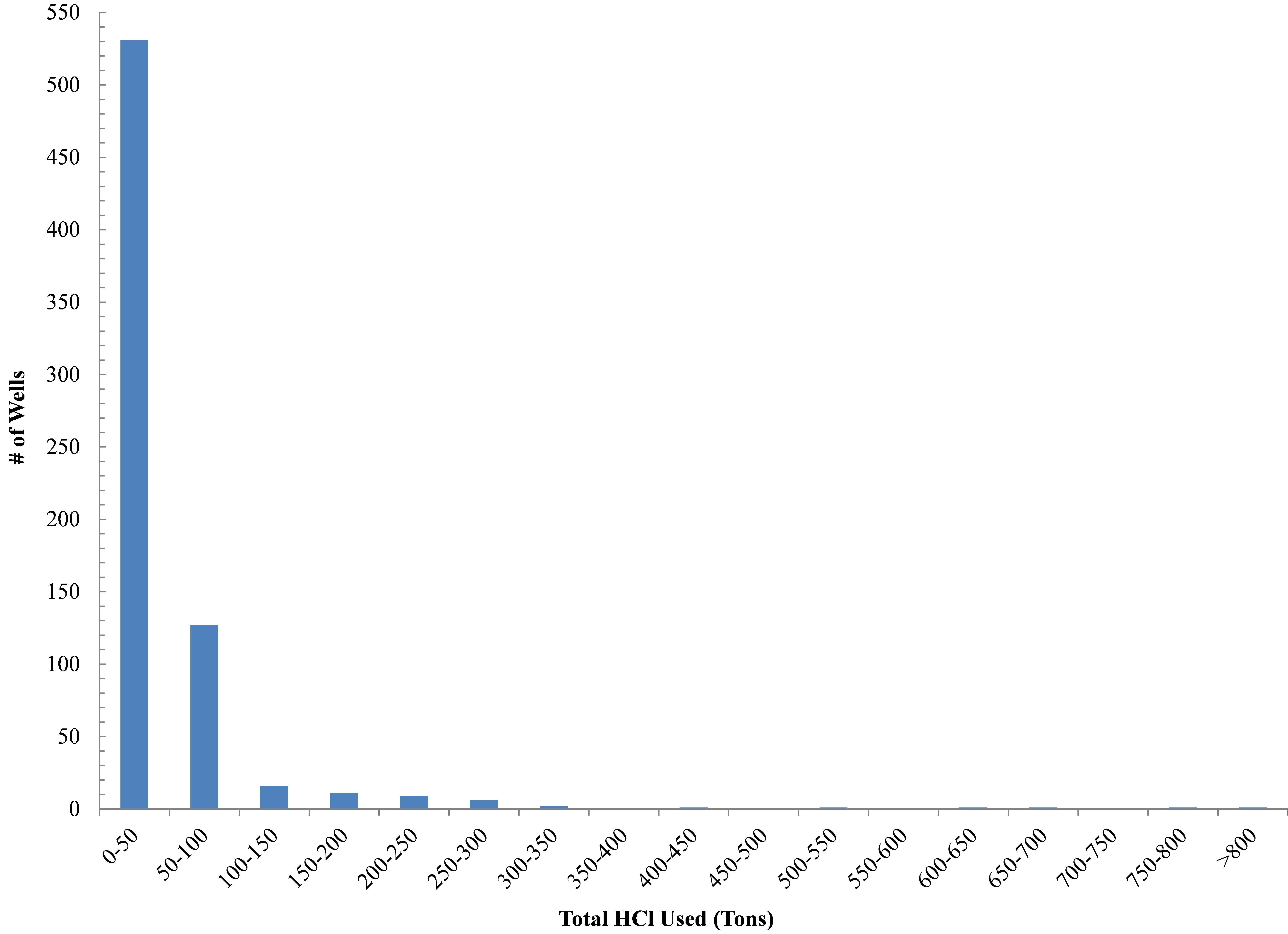
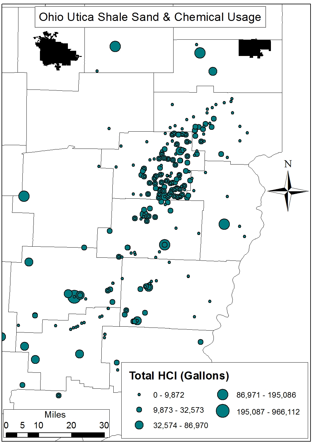
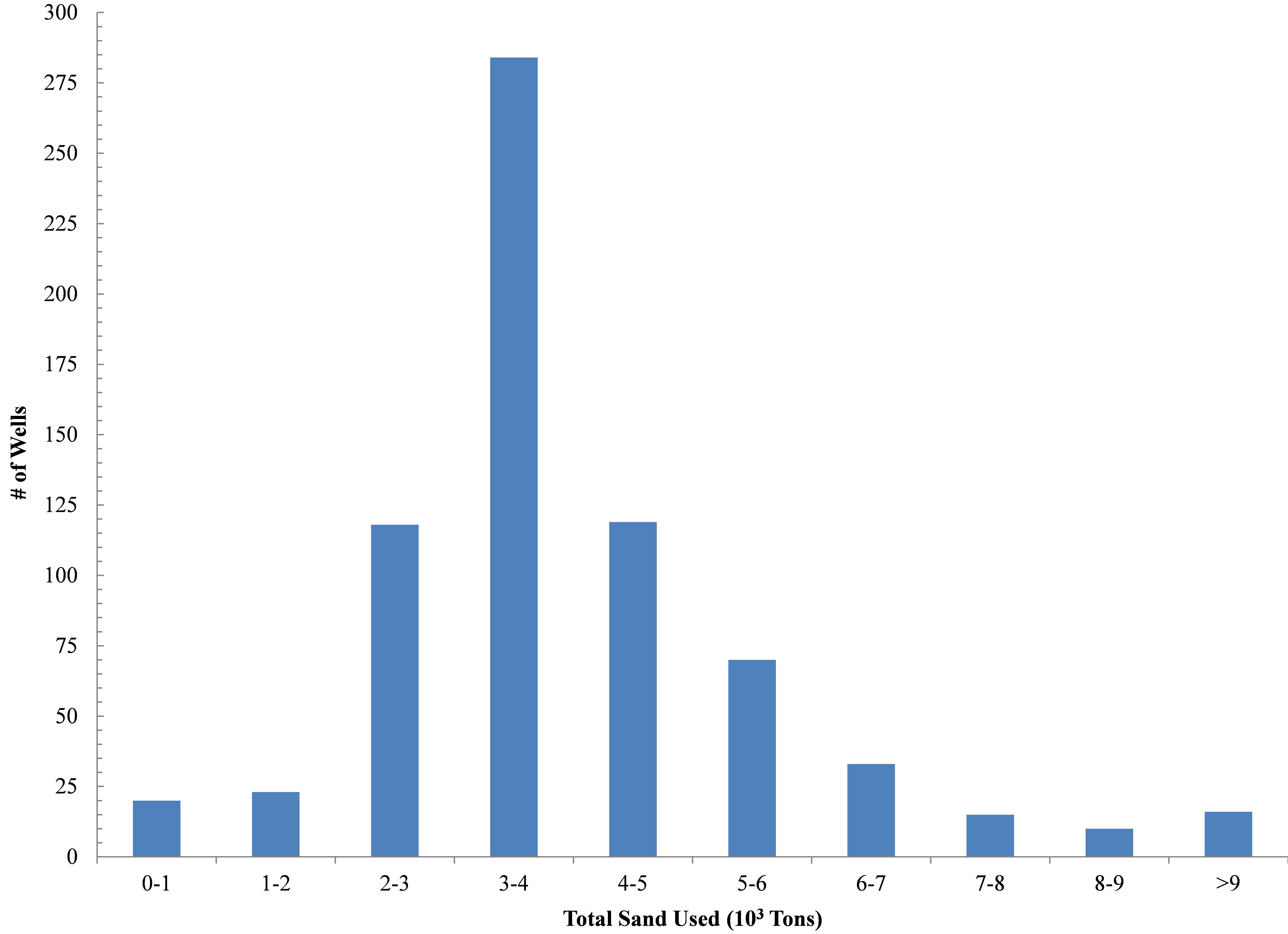
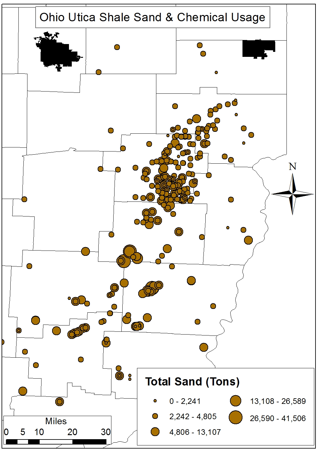
Figures 5a-d. Histograms and Spatial distribution of OH Utica Shale total hydrochloric acid (HCl, gallons) and silica sand (tons) demands.
Fig 5a. Histogram of OH Utica Shale total Hydrochloric Acid (HCl, gallons)
Fig 5b. Spatial distribution of OH Utica Shale total Hydrochloric Acid (HCl, gallons)
Fig 5c. Histogram of OH Utica Shale total Silica Sand (10^3 Tons)
Fig 5d. Spatial distribution of OH Utica Shale total Silica Sand (Tons)
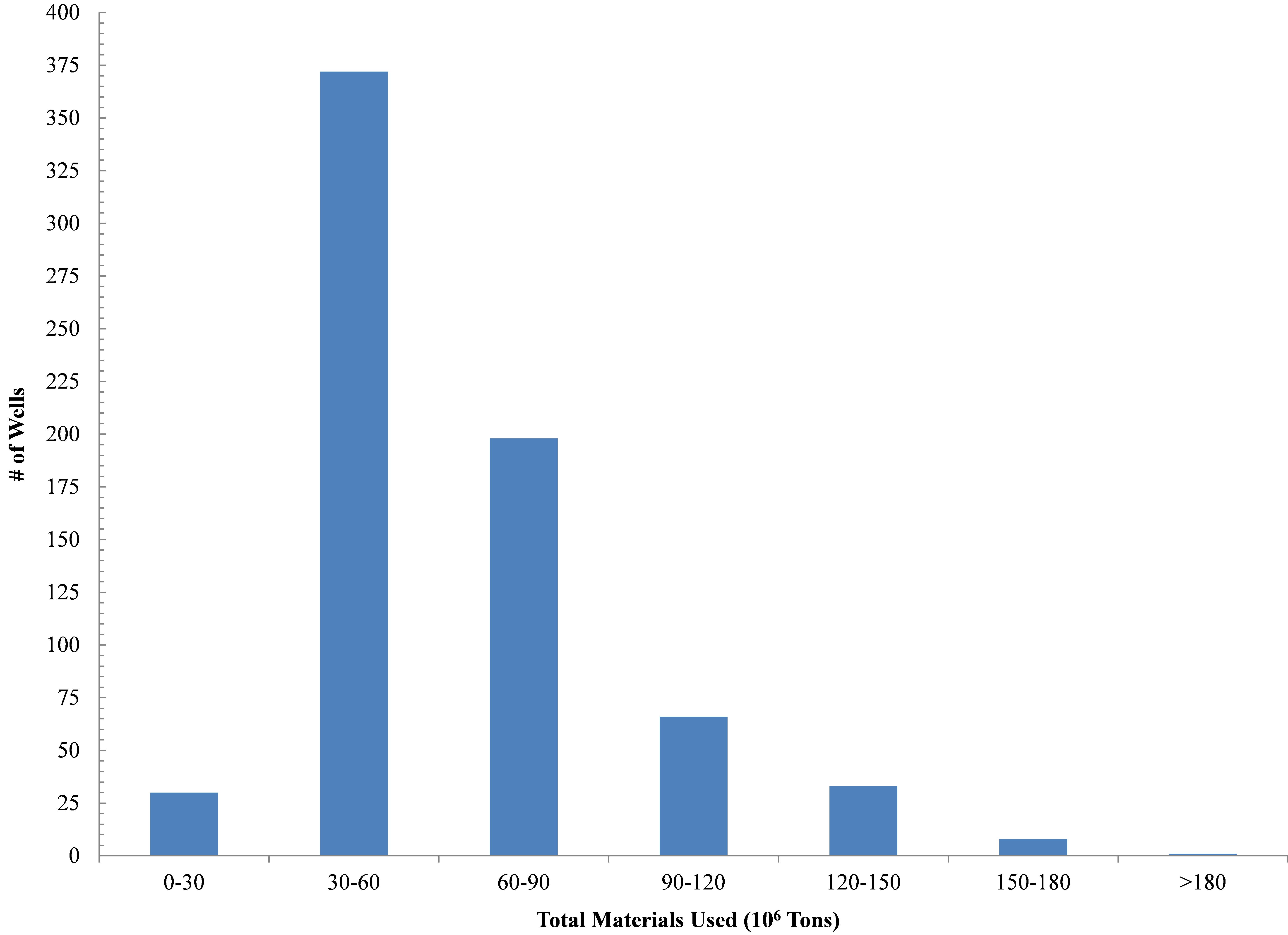
Figures 6a-b. Histograms and Spatial distribution of OH Utica Shale total resource utilization in terms of pounds per lateral.
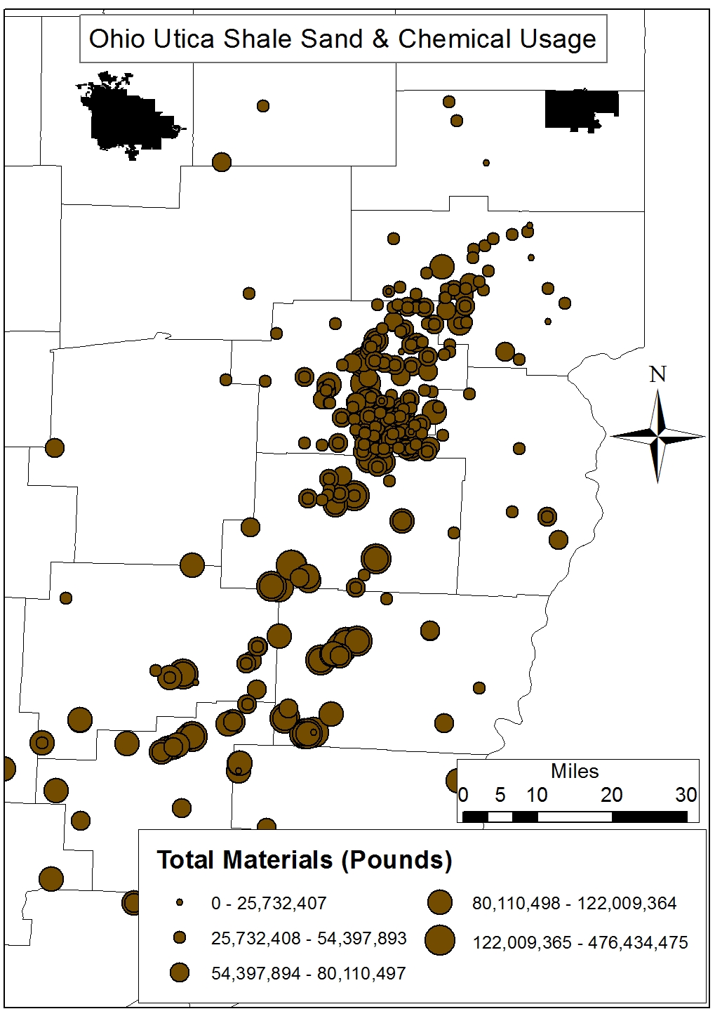
Fig 6a. Histogram of OH Utica Shale total materials used (10^6 Pounds)
Fig 6b. Spatial distribution of OH Utica Shale total materials used (Pounds)
Endnote
1. Additionally, all of Carroll County’s permitted wells lie within the already – and increasingly so – stressed Muskingum River Watershed (MRW) which has been a significant source of freshwater for the shale gas industry courtesy of the novel pricing schemes of its managing body the Muskingum Watershed Conservancy District (MWCD) (Figure 1). Carroll laterals are requiring 5.41 million gallons per lateral Vs the state average of 6.58 million gallons per lateral.
https://www.fractracker.org/a5ej20sjfwe/wp-content/uploads/2015/02/Carroll-Feature.jpg400900Ted Auch, PhDhttps://www.fractracker.org/a5ej20sjfwe/wp-content/uploads/2025/09/2025-Wordmark-Logo.pngTed Auch, PhD2015-02-16 15:47:382020-07-21 10:32:08Is Carroll Co. truly the king of Ohio’s Utica counties?
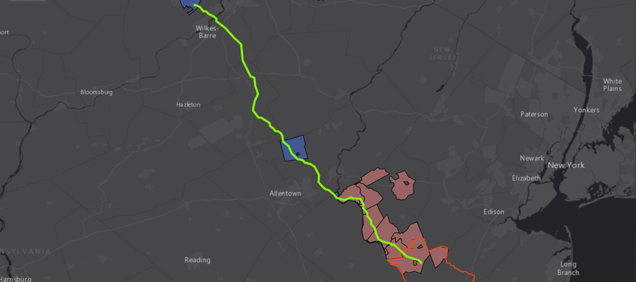
New York State is not the only area where opposition to fracking and its related activities is emerging. A 108-mile proposed PennEast pipeline between Wilkes-Barre, PA and Mercer County, New Jersey is facing municipal movements against its construction, as well. The 36-inch diameter pipeline will likely carry 1 billion cubic feet of natural gas per day. According to some sources, this proposed pipeline is the only one in NJ that is not in compliance with the state’s standard of co-locating new pipelines with an existing right-of-way.1
PennEast Pipeline Oppositions
Below is a dynamic, clickable map of said opposition by FracTracker’s Karen Edelstein, as well as documentation associated with each municipality’s current stance:
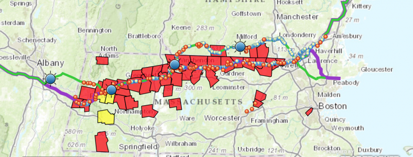
And in Massachusetts and New Hampshire, municipalities are working to ban, reroute, or regulate heavily the Northeast Energy Direct Pipeline (opposition map shown below):
Northeast Energy Direct Proposed Pipeline Paths and Opposition Resolutions in MA & NH
Why is this conversation important?
Participation in government is a beneficial practice for citizens and helps to inform our regulatory agencies on what people want and need. This surge in opposition against oil and gas activity such as pipelines or well pads near schools highlights a broader question, however:
If not pipelines, what is the least risky form of oil and gas transportation?
Oil and gas-related products are typically transported in one of four ways: Truck, Train, Barge, or Pipeline.
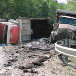
Drilling mud spill from truck accident
Lac-Mégantic oil train derailment
Using a barge to transport frac sand
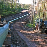
Gas pipeline construction in PA forest
Trucks are arguably the most risky and environmentally costly form of transport, with spills and wrecks documented in many communities. Because most of these well pads are being built in remote areas, truck transport is not likely to disappear anytime soon, however.
Transport by rail is another popular method, albeit strewn with incidents. Several, major oil train explosions and derailments, such as the Lac-Mégantic disaster in 2013, have brought this issue to the public’s attention recently.
Moving oil and gas products by barge is a different mode that has been received with some public concern. While the chance of an incident occurring could be lower than by rail or truck, using barges to move oil and gas products still has its own risks; if a barge fails, millions of people’s drinking water could potentially be put at risk, as highlighted by the 2014 Elk River chemical spill in WV.
So we are left with pipelines – the often-preferred transport mechanism by industry. Pipelines, too, bring with them explosion and leak potential, but at a smaller level according to some sources.2 Property rights, forest loss and fragmentation, sediment discharge into waterways, and the potential introduction of invasive species are but a few examples of the other concerns related to pipeline construction. Alas, none of the modes of transport are without risks or controversy.
Footnotes
Colocation refers to the practice of constructing two projects – such as pipelines – in close proximity to each other. Colocation typically reduces the amount of land and resources that are needed.
OH Utica Production, Water Usage, and Waste Disposal by County Part II of a Multi-part Series
By Ted Auch, Great Lakes Program Coordinator, FracTracker Alliance
In this part of our ongoing “Water-Energy Nexus” series focusing on Water and Water Use, we are looking at how counties in Ohio differ between how much oil and gas are produced, as well as the amount of water used and waste produced. This analysis also highlights how the OH DNR’s initial Utica projections differ dramatically from the current state of affairs. In the first article in this series, we conducted an analysis of OH’s water-energy nexus showing that Utica wells are using an ave. of 5 million gallons/well. As lateral well lengths increase, so does water use. In this analysis we demonstrate that:
Drillers have to use more water, at higher pressures, to extract the same unit of oil or gas that they did years ago,
Where production is relatively high, water usage is lower,
As fracking operations move to the perimeter of a marginally productive play – and smaller LLCs and MLPs become a larger component of the landscape – operators are finding minimal returns on $6-8 million in well pad development costs,
Market forces and Muskingum Watershed Conservancy District (MWCD) policy has allowed industry to exploit OH’s freshwater resources at bargain basement prices relative to commonly agreed upon water pricing schemes.
At current prices1, the shale gas industry is allocating < 0.27% of total well pad costs to current – and growing – freshwater requirements. It stands to reason that this multi-part series could be a jumping off point for a more holistic discussion of how we price our “endless” freshwater resources here in OH.
In an effort to better understand the inter-county differences in water usage, waste production, and hydrocarbon productivity across OH’s 19 Utica Shale counties we compiled a data-set for 500+ Utica wells which was previously used to look at differenced in these metrics across the state’s primary industry players. The results from Table 1 below are discussed in detail in the subsequent sections.
Table 1. Hydrocarbon production totals and per day values with top three producers in bold
County
# Wells
Total
Per Day
Oil
Gas
Brine
Production
Days
Oil
Gas
Brine
Ashland
1
0
0
23,598
102
0
0
231
Belmont
32
55,017
39,564,446
450,134
4,667
20
8,578
125
Carroll
256
3,715,771
121,812,758
2,432,022
66,935
67
2,092
58
Columbiana
26
165,316
9,759,353
189,140
6,093
20
2,178
65
Coshocton
1
949
0
23,953
66
14
0
363
Guernsey
29
726,149
7,495,066
275,617
7,060
147
1,413
49
Harrison
74
2,200,863
31,256,851
1,082,239
17,335
136
1,840
118
Jefferson
14
8,396
9,102,302
79,428
2,819
2
2,447
147
Knox
1
0
0
9,078
44
0
0
206
Mahoning
3
2,562
0
4,124
287
9
0
14
Medina
1
0
0
20,217
75
0
0
270
Monroe
12
28,683
13,077,480
165,424
2,045
22
7,348
130
Muskingum
1
18,298
89,689
14,073
455
40
197
31
Noble
39
1,326,326
18,251,742
390,791
7,731
268
3,379
267
Portage
2
2,369
75,749
10,442
245
19
168
228
Stark
1
17,271
166,592
14,285
602
29
277
24
Trumbull
8
48,802
742,164
127,222
1,320
36
566
100
Tuscarawas
1
9,219
77,234
2,117
369
25
209
6
Washington
3
18,976
372,885
67,768
368
59
1,268
192
Production
Total
It will come as no surprise to the reader that OH’s Utica oil and gas production is being led by Carroll County, followed distantly by Harrison, Noble, Belmont, Guernsey and Columbiana counties. Carroll has produced 3.7 million barrels of oil to date, while the latter have combined to produce an additional 4.5 million barrels. Carroll wells have been in production for nearly 67,000 days2, while the aforementioned county wells have been producing for 42,886 days. The remaining counties are home to 49 wells that have been in production for nearly 8,800 days or 7% of total production days in Ohio.
Combined with the state’s remaining 49 producing wells spread across 13 counties, OH’s Utica Shale has produced 8.3 million barrels of oil as well as 251,844,311 Mcf3 of natural gas and 5.4 million barrels of brine. Oil and natural gas together have an estimated value of $2.99 billion ($213 million per quarter)4 assuming average oil and natural gas prices of $96 per barrel and $8.67 per Mcf during the current period of production (2011 to Q2-2014), respectively.
Potential Revenue at Different Severance Tax Rates:
Current production tax, 0.5-0.8%: $19 million ($1.4 Million Per Quarter (MPQ). At this rate it would take the oil and gas industry 35 years to generate the $4.6 billion in tax revenue they proposed would be generated by 2020.
Proposed, 1% gas and 4% oil: At Governor Kasich’s proposed tax rate, $2.99 billion translates into $54 million ($3.9 MPQ). It would still take 21 years to return the aforementioned $4.6 billion to the state’s coffers.
The bottom-line is that a production tax of 11-25% or more ($24-53 MPQ) would be necessary to generate the kind of tax revenue proposed by the end of 2020. This type of O&G taxation regime is employed in the states of Alaska and Oklahoma.
From an outreach and monitoring perspective, effects on air and water quality are two of the biggest gaps in our understanding of shale gas from a socioeconomic, health, and environmental perspective. Pulling out a mere 1% from any of these tax regimes would generate what we’ll call an “Environmental Monitoring Fee.” Available monitoring funds would range between $194,261 and $1.8 million ($16 million at 55%). These monies would be used to purchase 2-21 mobile air quality devices and 10-97 stream quantity/quality gauges to be deployed throughout the state’s primary shale counties to fill in the aforementioned data gaps.
Per-Day Production
On a per-day oil production basis, Belmont and Columbiana (20 barrels per day (BPD)) are overshadowed by Washington (59 BPD) and Muskingum (40 BPD) counties’ four giant Utica wells. Carroll is able to maintain such a high level of production relative to the other 15 counties by shear volume of producing wells; Noble (268 BPD), Guernsey (147 BPD), and Harrison (136 BPD) counties exceed Carroll’s production on a per-day basis. The bottom of the league table includes three oil-free wells in Ashland, Knox, and Medina, as well as seventeen <10 BPD wells in Jefferson and Mahoning counties.
With respect to natural gas, Harrison (1,840 Mcf per day (MPD)) and Guernsey counties are replaced by Monroe (7,348 MPD) and Jefferson (2,447 MPD) counties’ 26 Utica wells. The range of production rates for natural gas is represented by the king of natural gas producers, Belmont County, producing 8,578 MPD on the high end and Mahoning and Coshocton counties in addition to the aforementioned oil dry counties on the low end. Four of the five oil- or gas-dry counties produce the least amount of brine each day (BrPD). Coshocton, Medina, and Noble county Utica wells are currently generating 267-363 barrels of BrPD, with an additional seven counties generating 100-200 BrPD. Only four counties – 1.2% of OH Utica wells – are home to unconventional wells that generate ≤ 30 BrPD.
Water Usage
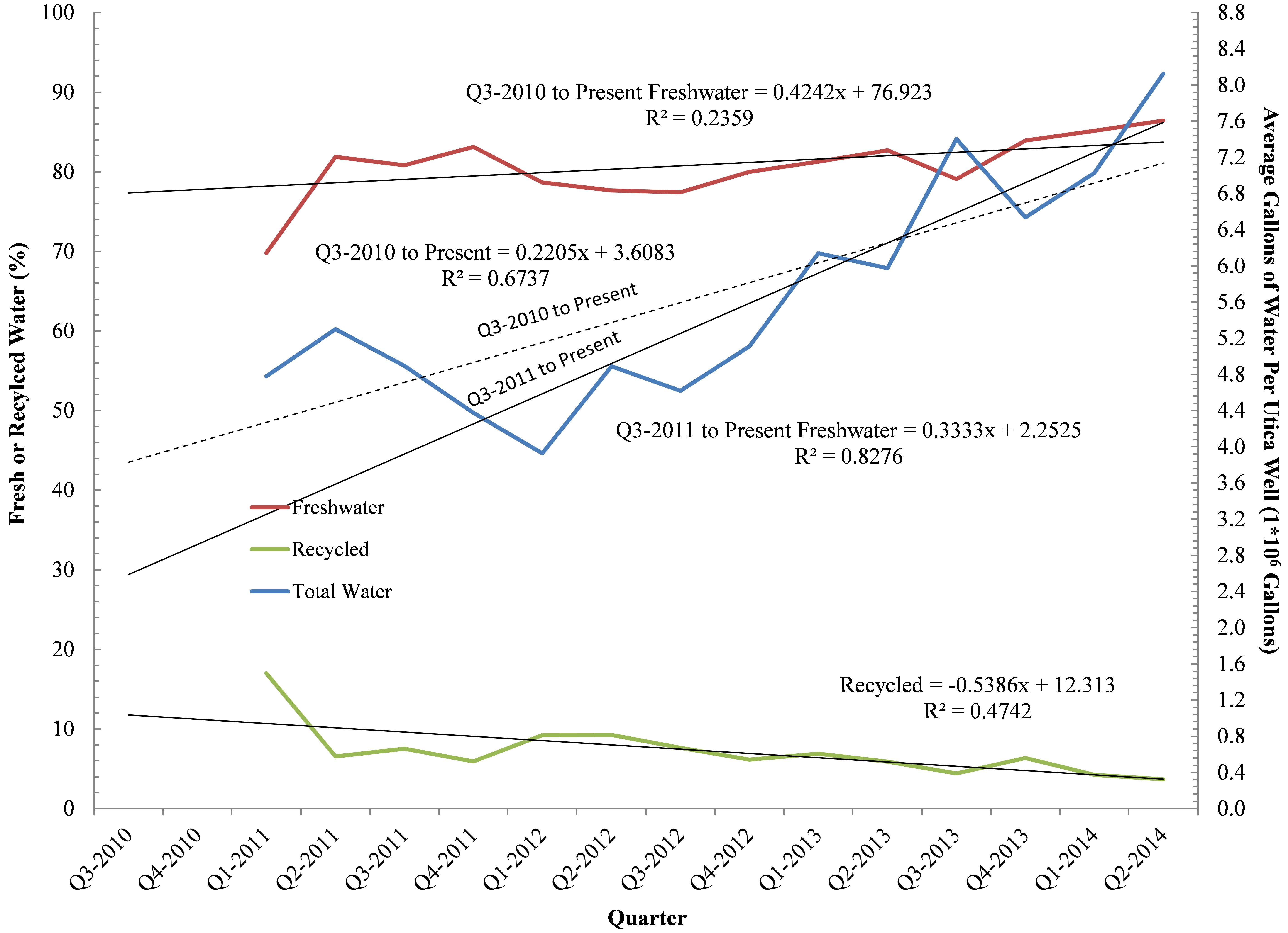
Freshwater is needed for the hydraulic fracturing process during well stimulation. For counties where we had compiled a respectable sample size we found that Monroe and Noble counties are home to the Utica wells requiring the greatest amount of freshwater to obtain acceptable levels of productivity (Figure 1). Monroe and Noble wells are using 10.6 and 8.8 million gallons (MGs) of water per well. Coshocton is home to a well that required 10.8 MGs, while Muskingum and Washington counties are home to wells that have utilized 10.2 and 9.5 MGs, respectively. Belmont, Guernsey, and Harrison reflect the current average state of freshwater usage by the Utica Shale industry in OH, with average requirements of 6.4, 6.9, and 7.2 MGs per well. Wells in eight other counties have used an average of 3.8 (Mahoning) to 5.4 MGs (Tuscarawas). The counties of Ashland, Knox, and Medina are home to wells requiring the least amount of freshwater in the range of 2.2-2.9 MGs. Overall freshwater demand on a per well basis is increasing by 220,500-333,300 gallons per quarter in Ohio with percent recycled water actually declining by 00.54% from an already trivial average of 6-7% in 2011 (Figure 2).
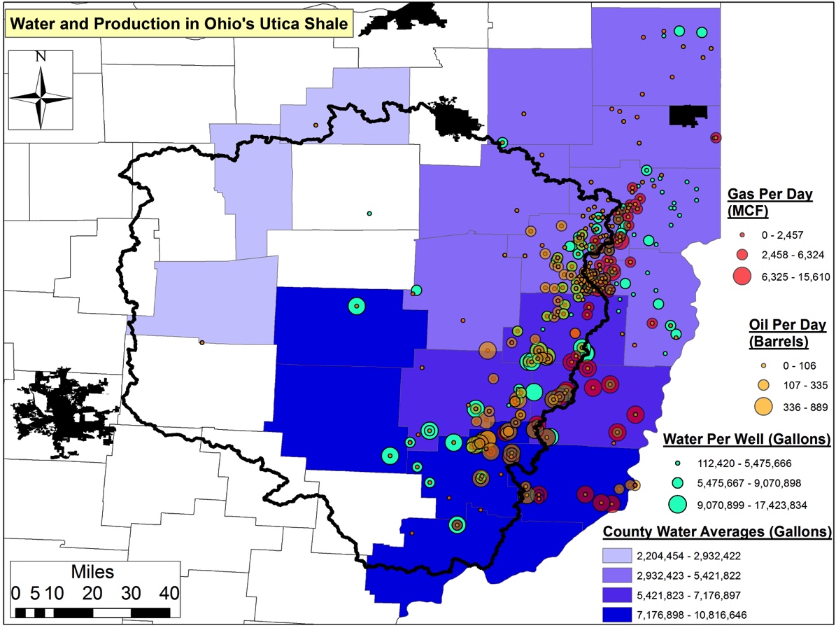
Figure 1. Average water usage (gallons) per Utica well by county
Figure 2. Average water usage (gallons) on per well basis by OH Utica Shale industry, shown quarterly between Q3-2010 & Q2-2014.
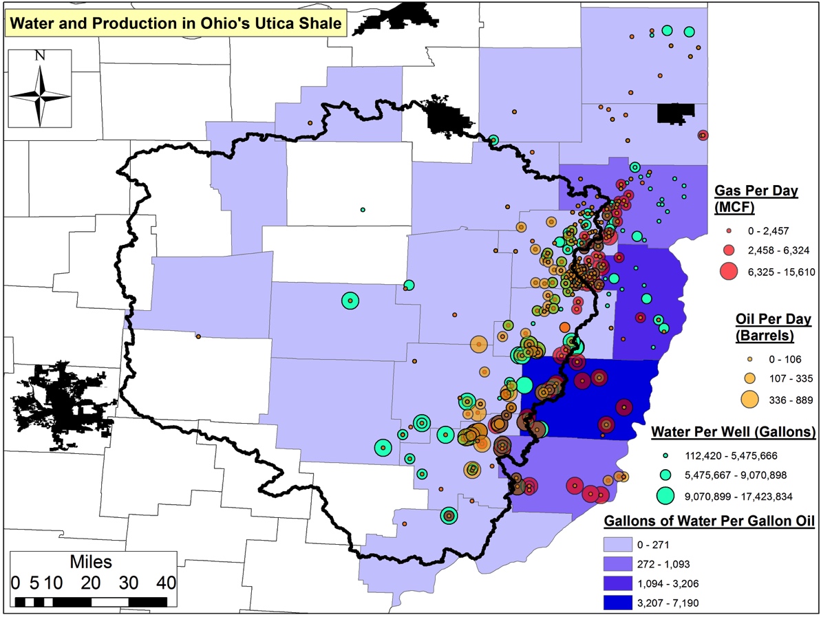
Belmont County’s 30+ Utica wells are the least efficient with respect to oil recovery relative to freshwater requirements, averaging 7,190 gallons of water per gallon of oil (Figure 3). A distant second is Jefferson County’s 14 wells, which have required on average 3,205 gallons of water per gallon of oil. Columbiana’s 26 Utica wells are in third place requiring 1,093 gallons of freshwater. Coshocton, Mahoning, Monroe, and Portage counties are home to wells requiring 146-473 gallons for each gallon of oil produced.
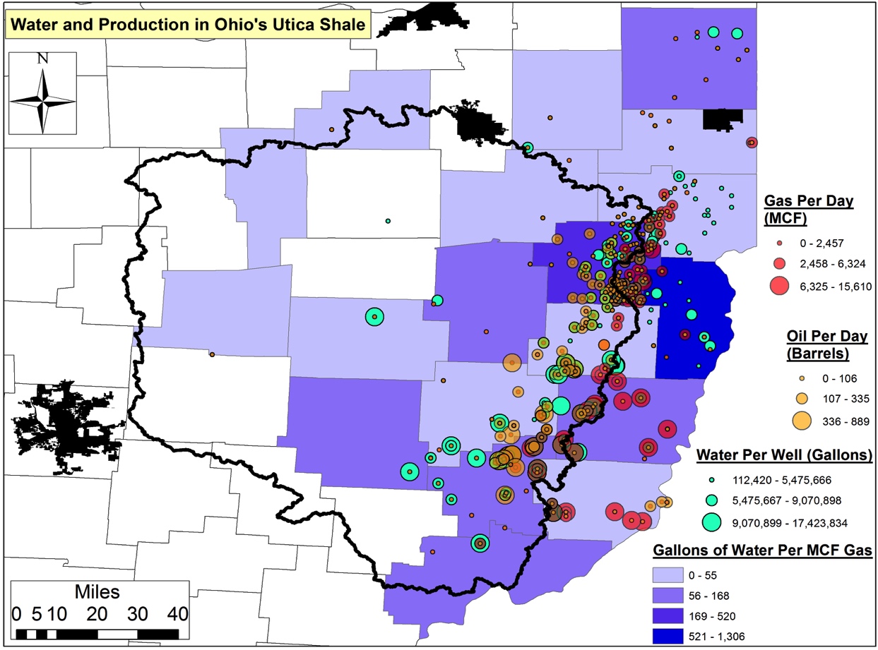
Belmont County’s 14 Utica wells are the least efficient with respect to natural gas recovery relative to freshwater requirements (Figure 4). They average 1,306 gallons of water per Mcf. A distant second is Carroll County’s 250+ wells, which have injected 520 gallons of water 7,000+ feet below the earth’s service to produce a single Mcf of natural gas. Muskingum’s Utica well and Noble County’s 39 wells are the only other wells requiring more than 100 gallons of freshwater per Mcf. The remaining nine counties’ wells require 15-92 gallons of water to produce an Mcf of natural gas.
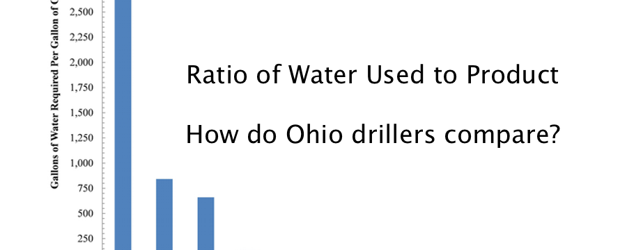
Figure 3. Average water usage (gallons) per unit of oil (gallons) produced across 19 Ohio Utica counties
Figure 4. Average water usage (gallons) per unit of gas produced (Mcf) across 19 Ohio Utica counties
Waste Production
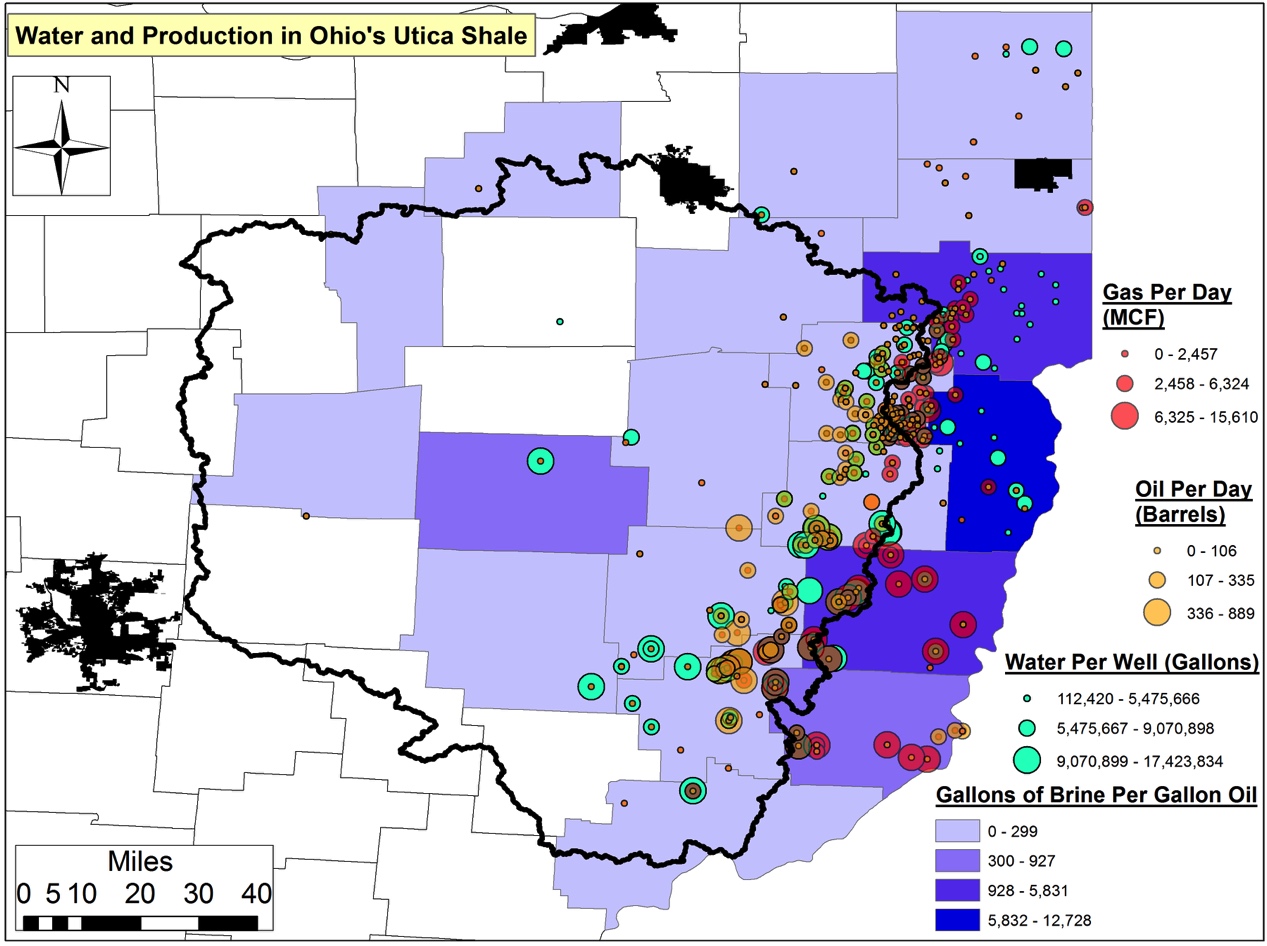
The aforementioned Jefferson wells are the least efficient with respect to waste vs. product produced. Jefferson wells are generating 12,728 gallons of brine per gallon of oil (Figure 5).6 Wells from this county are followed distantly by the 32 Belmont and 26 Columbiana county wells, which are generating 5,830 and 3,976 gallons of brine per unit of oil.5 The remaining counties (for which we have data) are using 8-927 gallons of brine per unit of oil; six counties’ wells are generating <38 gallons of brine per gallon of oil.
Figure 5. Average brine production (gallons) per gallon of oil produced per day across 19 Ohio Utica Counties
The average Utica well in OH is generating 820 gallons of fracking waste per unit of product produced. Across all OH Utica wells, an average of 0.078 gallons of brine is being generated for every gallon of freshwater used. This figure amounts to a current total of 233.9 MGs of brine waste produce statewide. Over the next five years this trend will result in the generation of one billion gallons (BGs) of brine waste and 12.8 BGs of freshwater required in OH. Put another way…
233.9 MGs is equivalent to the annual waste production of 5.2 million Ohioans – or 45% of the state’s current population.
Due to the low costs incurred by industry when they choose to dispose of their fracking waste in OH, drillers will have only to incur $100 million over the next five years to pay for the injection of the above 1.0 BGs of brine. Ohioans, however, will pay at least $1.5 billion in the same time period to dispose of their municipal solid waste. The average fee to dispose of every ton of waste is $32, which means that the $100 million figure is at the very least $33.5 million – and as much as $250.6 million – less than we should expect industry should be paying to offset the costs.
Environmental Accounting
In summary, there are two ways to look at the potential “energy revolution” that is shale gas:
Using the same traditional supply-side economics metrics we have used in the past (e.g., globalization, Efficient Market Hypothesis, Trickle Down Economics, Bubbles Don’t Exist) to socialize long-term externalities and privatize short-term windfall profits, or
We can begin to incorporate into the national dialogue issues pertaining to watershed resilience, ecosystem services, and the more nuanced valuation of our ecosystems via Ecological Economics.
The latter will require a more real-time and granular understanding of water resource utilization and fracking waste production at the watershed and regional scale, especially as it relates to headline production and the often-trumpeted job generating numbers.
We hope to shed further light on this new “environmental accounting” as it relates to more thorough and responsible energy development policy at the state, federal, and global levels. The life cycle costs of shale gas drilling have all too often been ignored and can’t be if we are to generate the types of energy our country demands while also stewarding our ecosystems. As Mark Twain is reported to have said “Whiskey is for drinking; water is for fighting over.” In order to avoid such a battle over the water-energy nexus in the long run it is imperative that we price in the shale gas industry’s water-use footprint in the near term. As we have demonstrated so far with this series this issue is far from settled here in OH and as they say so goes Ohio so goes the nation!
A Moving Target
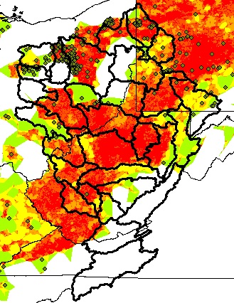
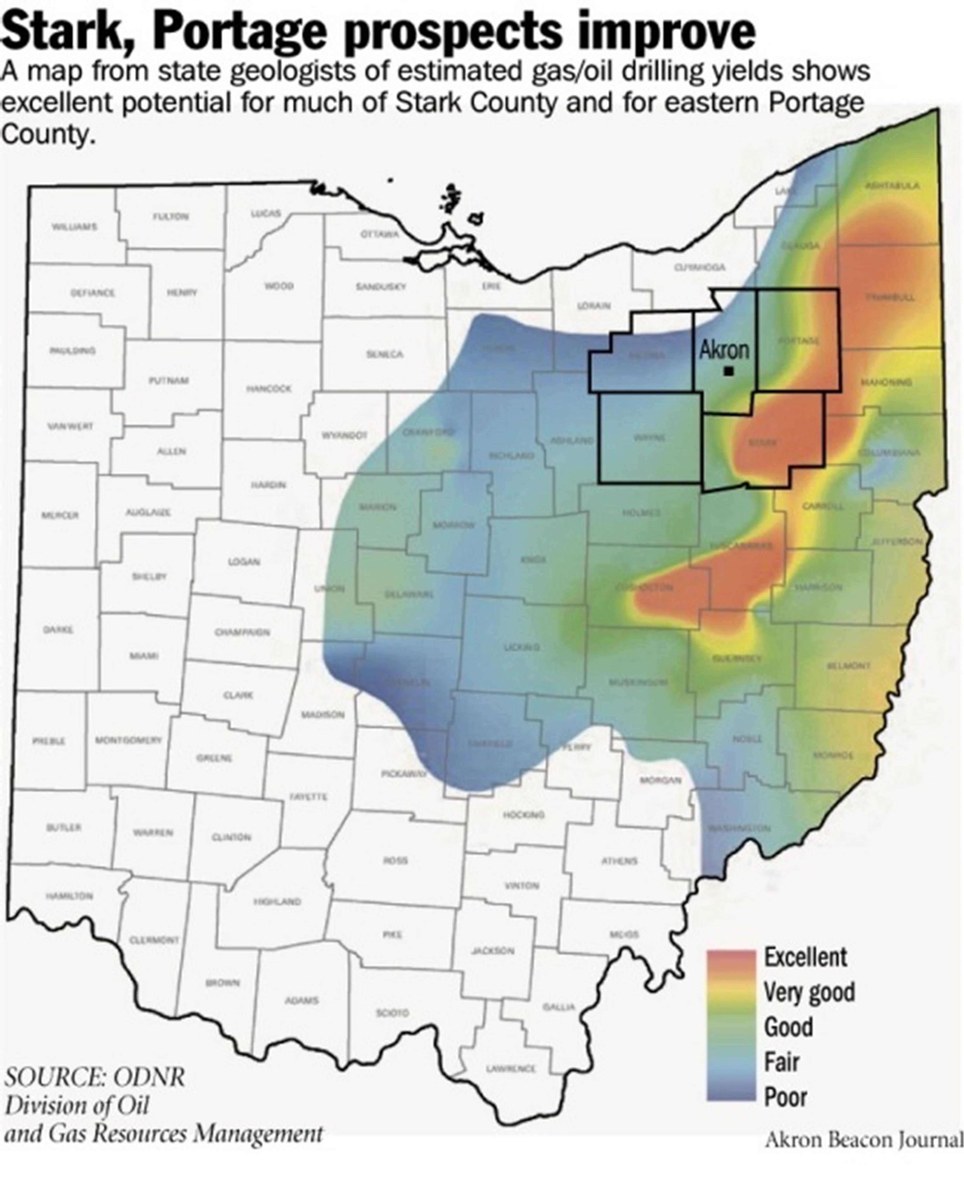
Figure 6. ODNR projection map of potential Utica productivity from spring 2012
OH’s Department of Natural Resources (ODNR) originally claimed a big red – and nearly continuous – blob of Utica productivity existed. The projection originally stretched from Ashtabula and Trumbull counties south-southwest to Tuscarawas, Guernsey, and Coshocton along the Appalachian Plateau (See Figure 6).
However, our analysis demonstrates that (Figures 7 and 8):
This is a rapidly moving target,
The big red blob isn’t as big – or continuous – as once projected, and
It might not even include many of the counties once thought to be the heart of the OH Utica shale play.
This last point is important because counties, families, investors, and outside interests were developing investment and/or savings strategies based on this map and a 30+ year timeframe – neither of which may be even remotely close according to our model.
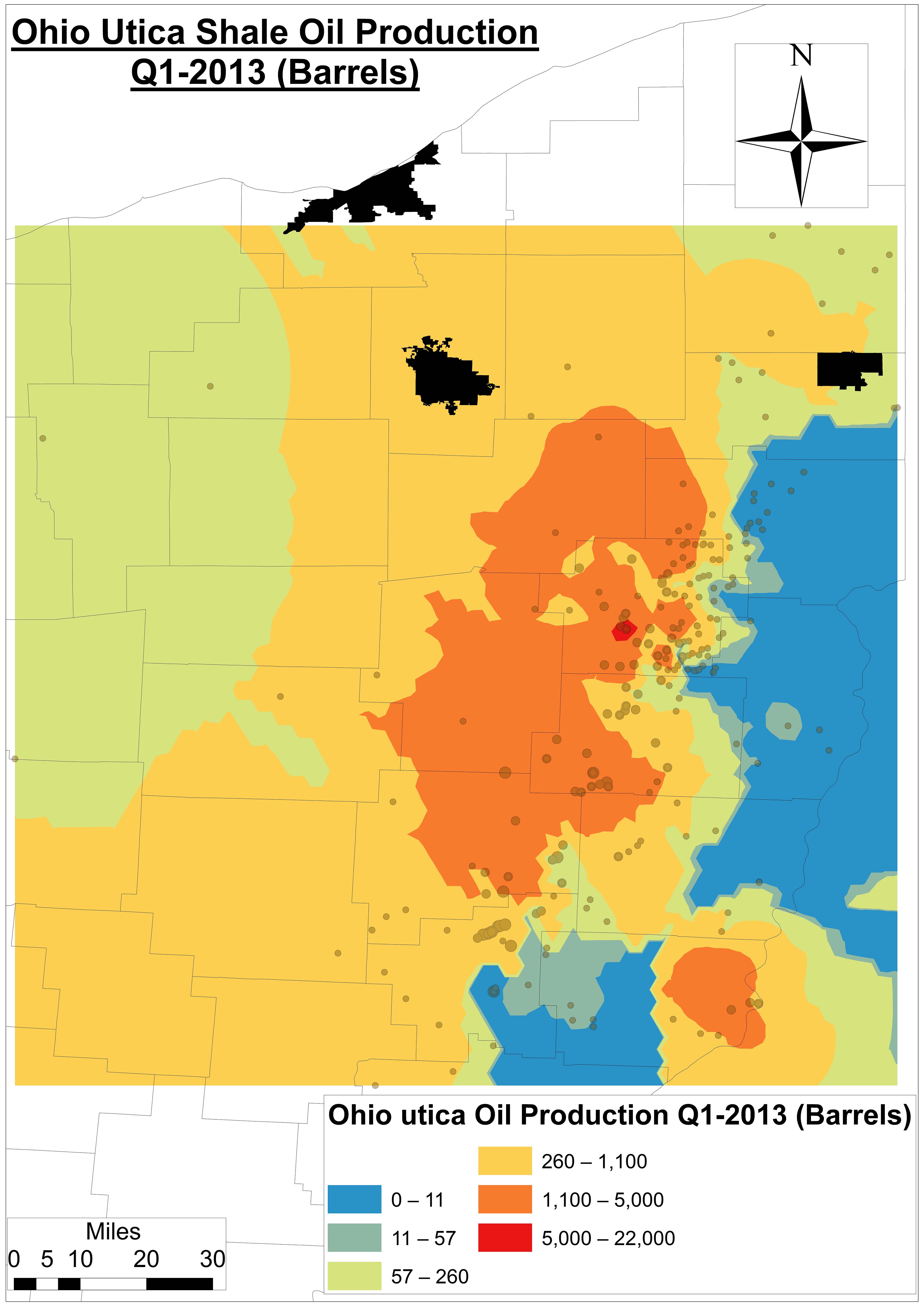
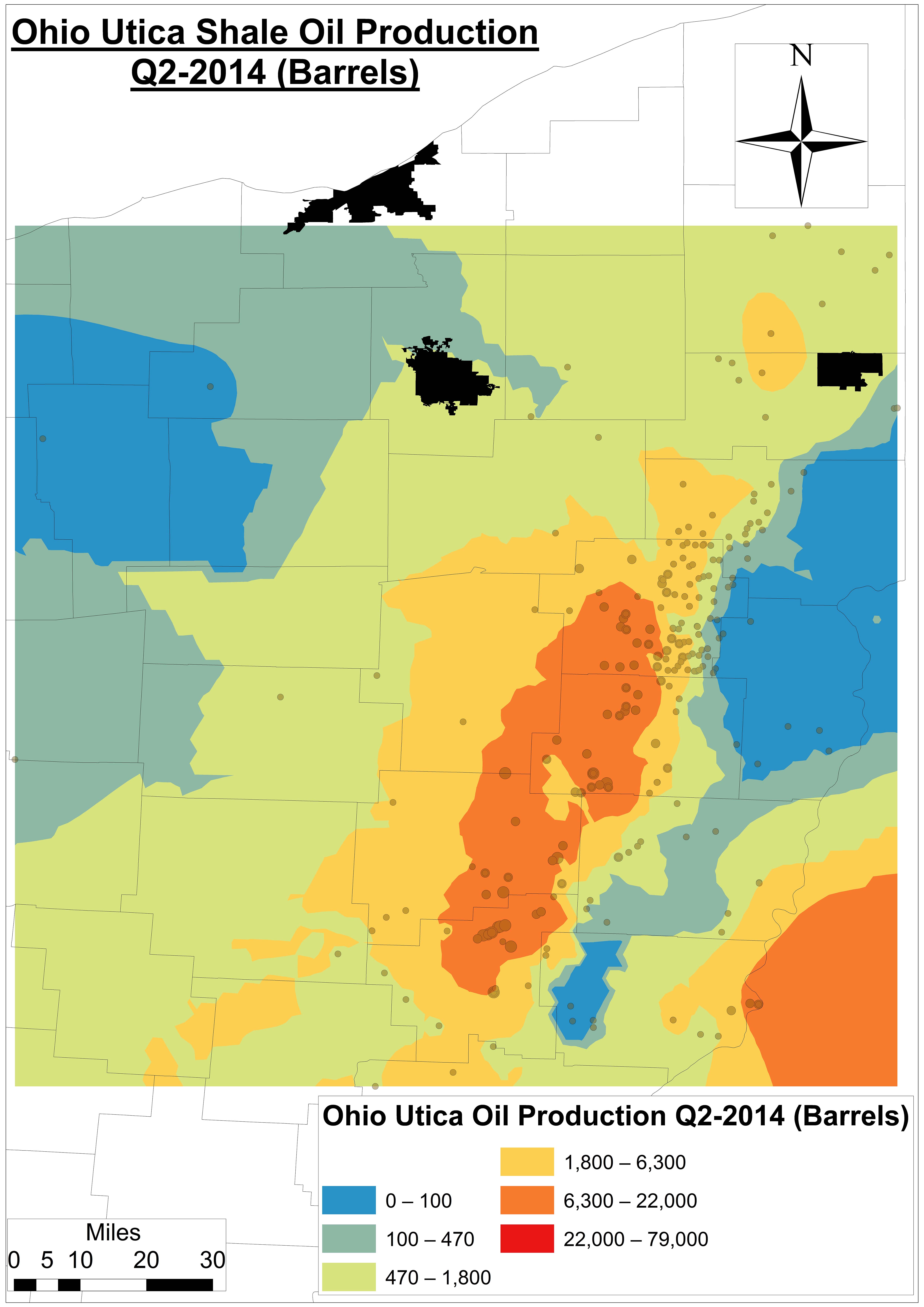
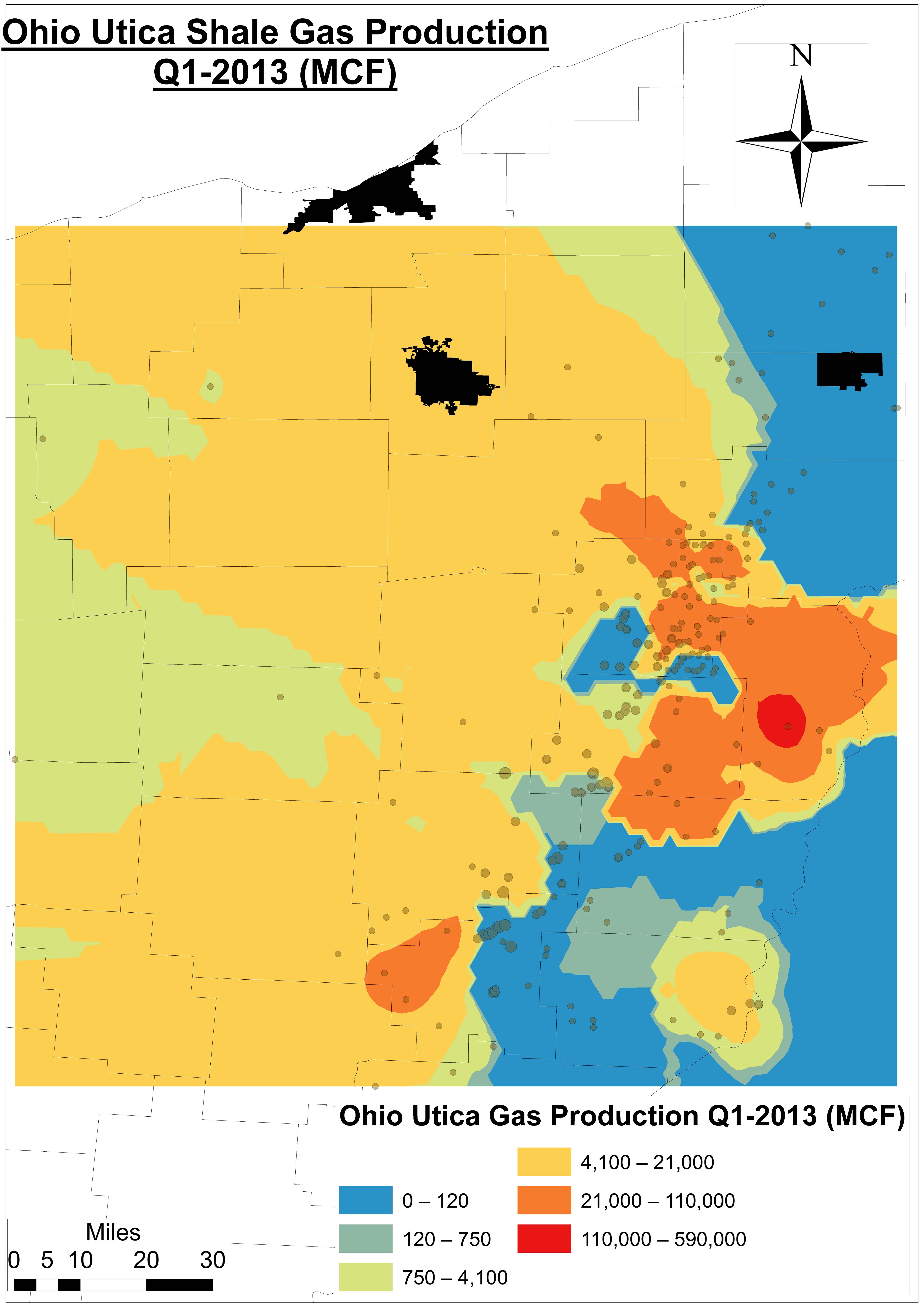
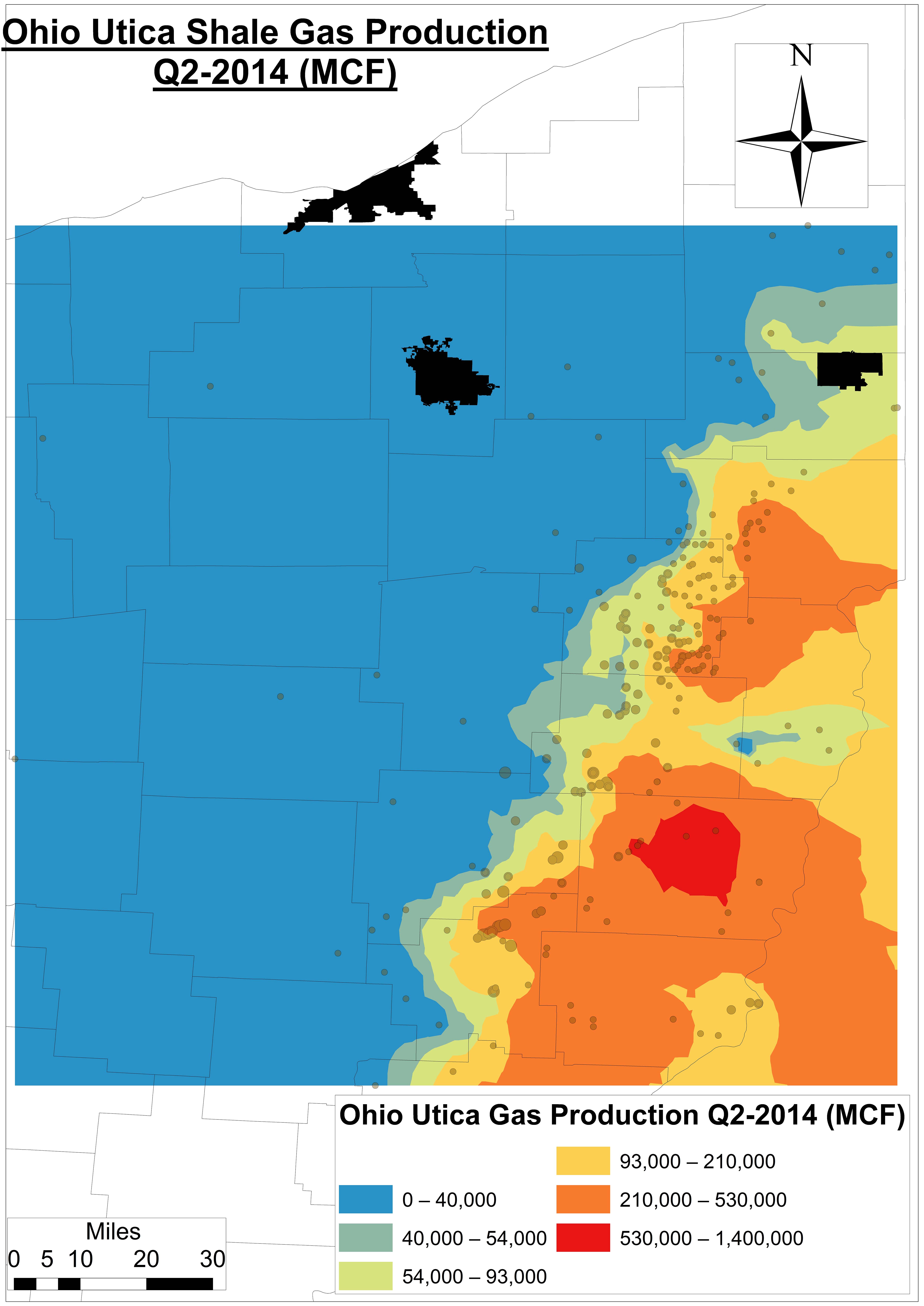
Figure 7a. An Ohio Utica Shale oil production model using Kriging6 for Q1-2013
Figure 7b. An Ohio Utica Shale oil production model using Kriging for Q2-2014
Figure 8a. An Ohio Utica Shale gas production model using Kriging for Q1-2013
Figure 8b. An Ohio Utica Shale gas production model using Kriging for Q2-2014
Footnotes
$4.25 per 1,000 gallons, which is the current going rate for freshwater at OH’s MWCD New Philadelphia headquarters, is 4.7-8.2 times less than residential water costs at the city level according to Global Water Intelligence.
Carroll County wells have seen days in production jump from 36-62 days in 2011-2012 to 68-78 in 2014 across 256 producing wells as of Q2-2014.
One Mcf is a unit of measurement for natural gas referring to 1,000 cubic feet, which is approximately enough gas to run an American household (e.g. heat, water heater, cooking) for four days.
Assuming average oil and natural gas prices of $96 per barrel and $8.67 per Mcf during the current period of production (2011 to Q2-2014), respectively
On a per-API# basis or even regional basis we have not found drilling muds data. We do have it – and are in the process of making sense of it – at the Solid Waste District level.
https://www.fractracker.org/a5ej20sjfwe/wp-content/uploads/2014/11/Nexus2-Feature.png400900Ted Auch, PhDhttps://www.fractracker.org/a5ej20sjfwe/wp-content/uploads/2025/09/2025-Wordmark-Logo.pngTed Auch, PhD2014-11-17 17:00:262020-07-21 10:34:07The Water-Energy Nexus in Ohio, Part II
OH Utica Production, Water Usage, and Changes in Lateral Length
Part I of a Multi-part Series By Ted Auch, OH Program Coordinator, FracTracker Alliance
As shale gas expands in Ohio, how too does water use? We conducted an analysis of 500+ Utica wells in an effort to better understand the water-energy nexus in Ohio between production, water usage, and lateral length across 500+ Utica wells. The following is a list of the primary findings from this analysis:
Lateral Length
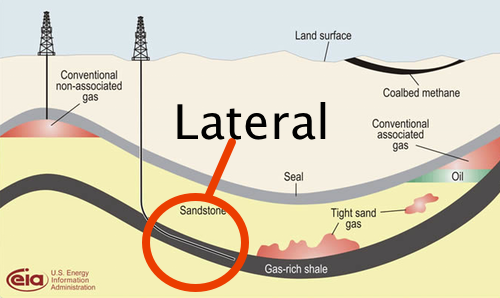
Figure 1. Modified EIA schematic highlighting the lateral portion of the unconventional well
In unconventional oil and gas drilling, often operators need to drill both vertically and then laterally to follow the formation underground. This process increases the amount of shale that the well contacts (see the modified EIA schematic in Figure 1). As a general rule Ohio’s Utica wells transition to the horizontal or lateral phase at around 6,800 feet below the earth’s surface.
1. The average Utica lateral is increasing in length by 51-55 feet per quarter, up from an average of 6,369 feet between Q3-2010 and Q2-2011 to 6,872 feet in the last four quarters. Companies’ lateral length growth varies, for example:
Gulfport is increasing by 46 feet (+67,206 gallons of water),
R.E. Gas Development and Antero 92 feet (+134,412 gallons of water), and
Chesapeake 28 feet (+40,908 gallons of water).
2. An increase in lateral length accounts for 40% of the increase in the water usage, as we have discussed in the past.
3. As a general rule, every foot increase in lateral length equates to an increase of 1,461 gallons of freshwater.
Regional and County-Level Trends
This section looks into big picture of shale gas drilling in OH. Herein we summarize the current state of water usage by the Utica shale industry relative to hydrocarbon production, as a percentage of residential water usage, as well as long-term water usage and waste production forecasts.
1. Freshwater Use
Across 516 wells, we found that the average OH Utica well utilizes 5.04-5.69 million gallons of freshwater per well.
This figure includes a ratio of 12:1 freshwater to recycled water used on site.
Water usage is increasing by 221-330,000 gallons per well per quarter.
Note: In neighboring – and highly OH freshwater reliant-West Virginia, the average Marcellus well uses 6.1-6.6 million gallons per well, with a trend increase of 189-353,000 gallons per quarter per well.
Water usage is up from 4.88 million gallons per well between 2010 and the summer of 2011 to 7.27 million gallons today.
Over the next five years, we will likely see 18.5 billion gallons of freshwater used for shale gas drilling in OH.
On average, drilling companies use 588 gallons of water to get a gallon of oil.
Average: 338 gallons of water required to get 1 MCF of gas
Average: 0.078 gallons of brine produced per gallon of water
2. Residential Water Allocation
A portion of residential water (3.8-6.1% of usage) is being allocated to the Utica drilling boom.
This figure is as high as 81% of residential water requirements in Carroll County.
And amounts to 2.2-3.5% of the available water in the Muskingum River Watershed.
The allocation will increase over time to amount to 8.2-10.5% of residential usage or 4.4-5.6% of Muskingum River available water.
3. Permitted Wells Potential
If all permitted Utica wells were to come online (active), we could expect 299.7 million gallons of additional brine to be produced and an additional 220 million gallons of freshwater a year to be used.
This trend amounts to 1.1 billion gallons of fracking brine waste looking for a home within 5 years.
4. Waste Disposal
Stallion Oilfield Services has recently purchased several Class II Injection wells in Portage County.
These waste disposal sites are increasing their intake at a rate of 2.13 million gallons per quarter, 4.76 times that of the rest of OH Class II wells.
Water Usage By Company
The data trends we have reviewed vary significantly depending on the company that is assessed. Below we summarize the current state of water usage by the major players in Ohio’s Utica shale industry relative to hydrocarbon production.
1. Overall Statistics
The 15 biggest Water-To-Oil offenders are currently averaging 16,844 Gallons of Water per gallon of oil (PGO) (i.e., Shugert 2-12H, Salem-Grubbs 1H, Stutzman 1 and 3-14H, etc).
Removing the above 15 brings the Water-To-Oil ratio down from 588 to 52 gallons of water PGO.
The 9 biggest Water-To-Gas offenders are currently averaging 16,699 gallons of water per MCF of gas.
Removing the above 9 brings the Water-To-Gas ratio down from 338 to 27 gallons of water per MCF of gas.
Company differences are noticeable (Figure 2):
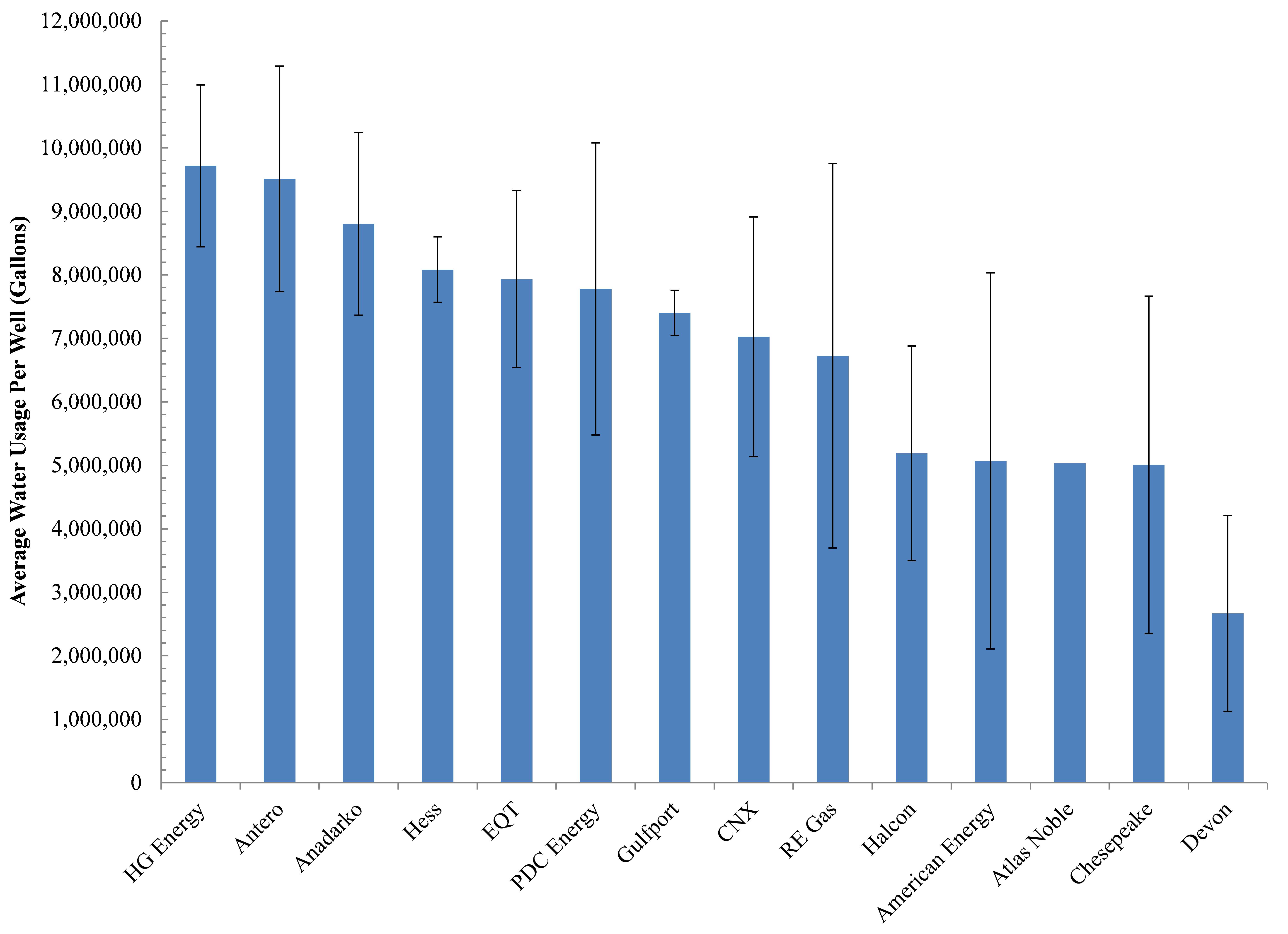
Figure 2. Average Freshwater Use Among OH Utica Operators
Antero and Anadarko used an average of 9.5 and 8.8 MGs of water per well during the course of the 45-60 drilling process, respectively (Note: HG Energy has the wells with the highest water usage but a limited sample size, with 9.8 MGs per well).
Six companies average in the middle with 6.7-8.1 MGs of water per well.
Four companies average 5 MGs per well, including Chesapeake the biggest player here in OH.
Devon Energy is the one firm using less than 3 MGs of freshwater for each well it drills.
2. Water-to-Oil Ratios
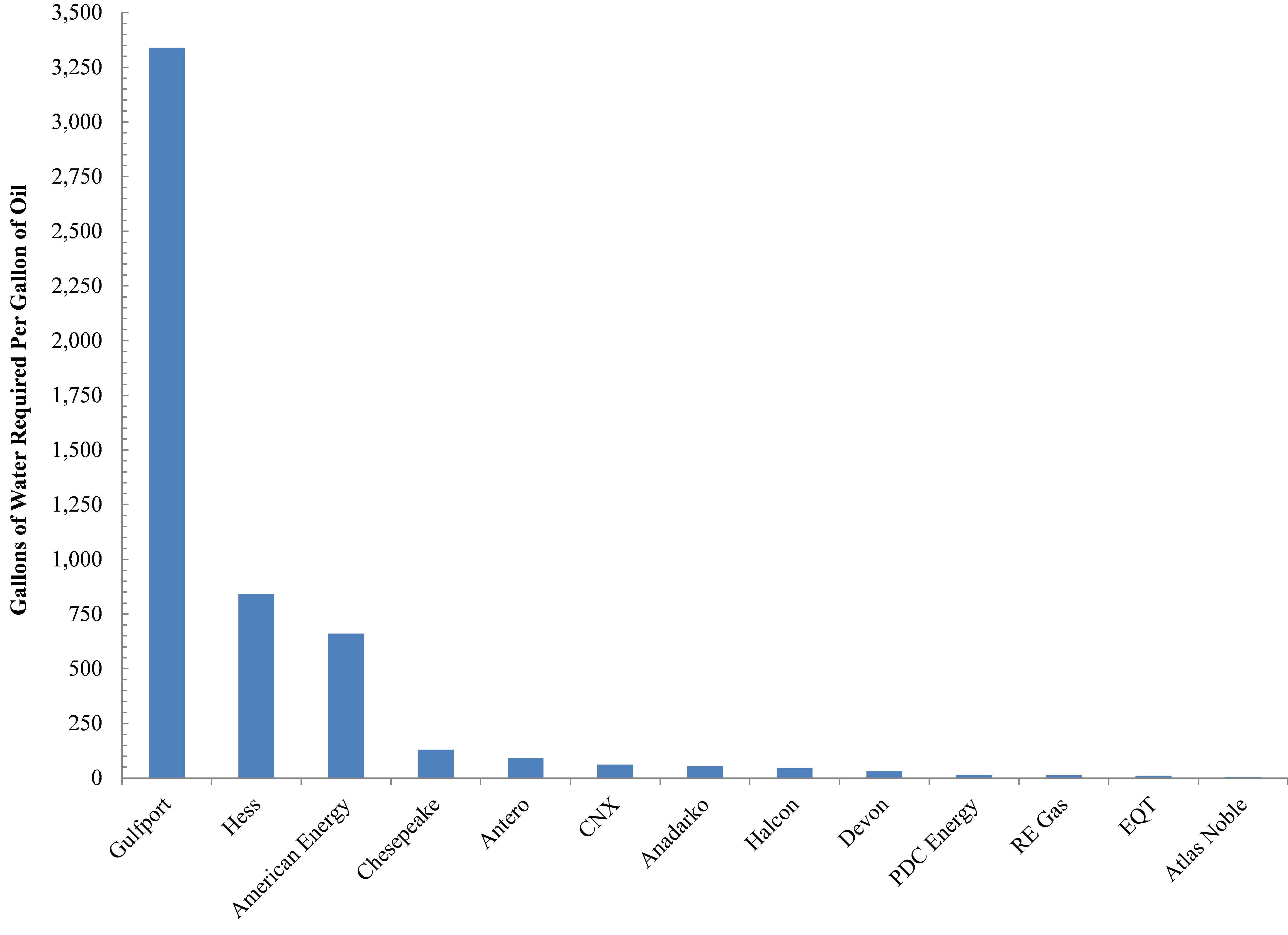
Figure 3. Water-to-Oil Ratios Among OH Utica Operators
Freshwater usage is increasing by 3.6 gallons per gallon of oil. Companies vary less in this metric, except for Gulfport (Figure 3):
Gulfport is by far the least efficient user of freshwater with respect to oil production, averaging 3,339 gallons of water to extract one gallon of oil.
Intermediate firms include American Energy and Hess, which required 661 and 842 gallons of freshwater to produce a gallon of oil.
The remaining eleven firms used anywhere from 6 (Atlas Noble) to 130 (Chesapeake) gallons of freshwater to get a unit of oil.
3. Water-to-Gas Ratios (Figure 4)
Figure 4. Water-to-Gas Ratio Among OH Utica Operators
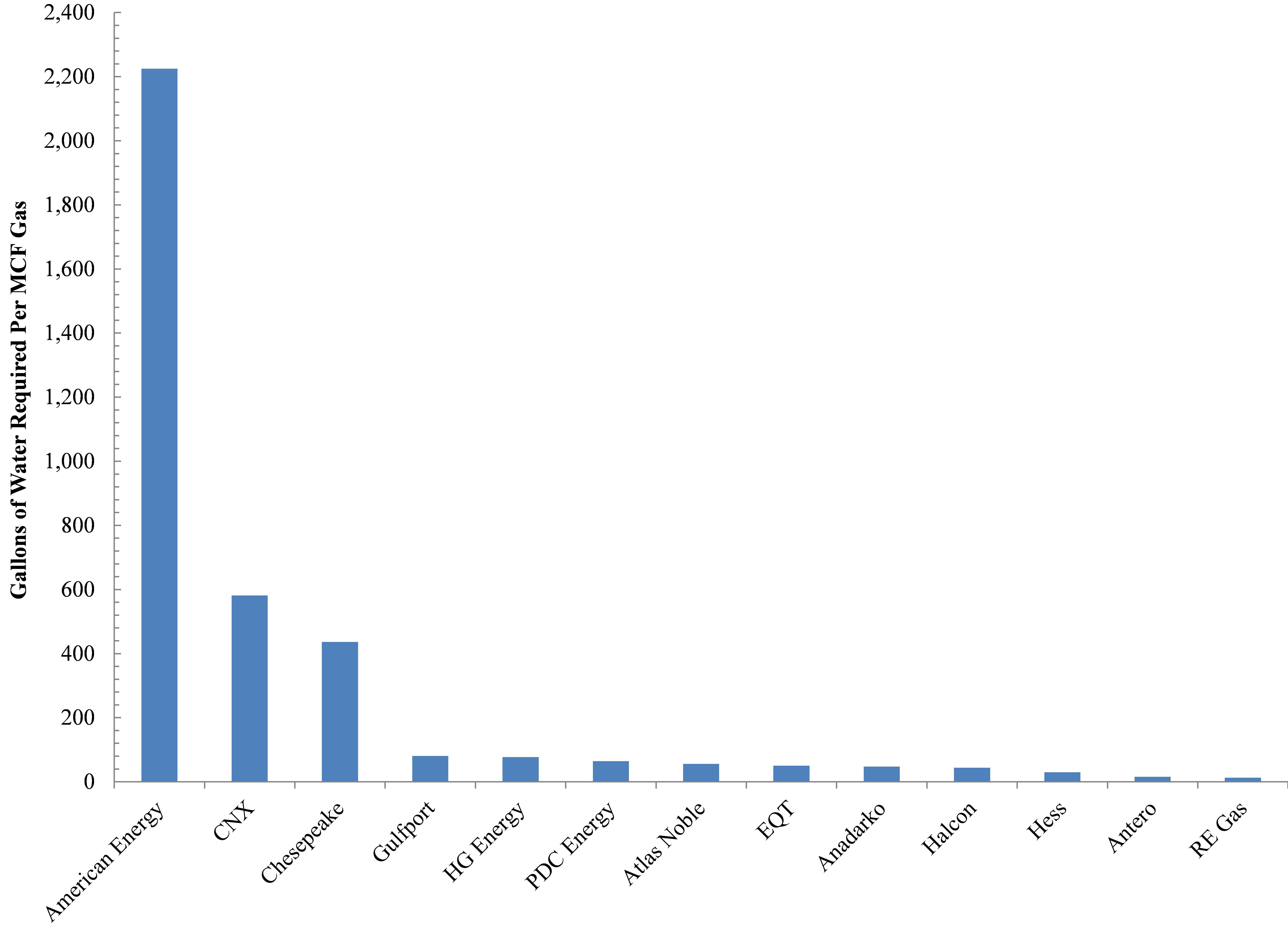
American Energy is also quite inefficient when it comes to natural gas production utilizing >2,200 gallons of freshwater per MCF of natural gas produced
Chesapeake and CNX rank a distant second, requiring 437 and 582 gallons of freshwater per MCF of natural gas, respectively.
The remaining firms for which we have data are using anywhere from 13 (RE Gas) to 81 (Gulfport) gallons of freshwater per MCF of natural gas.
4. Brine Production (Figure 5)
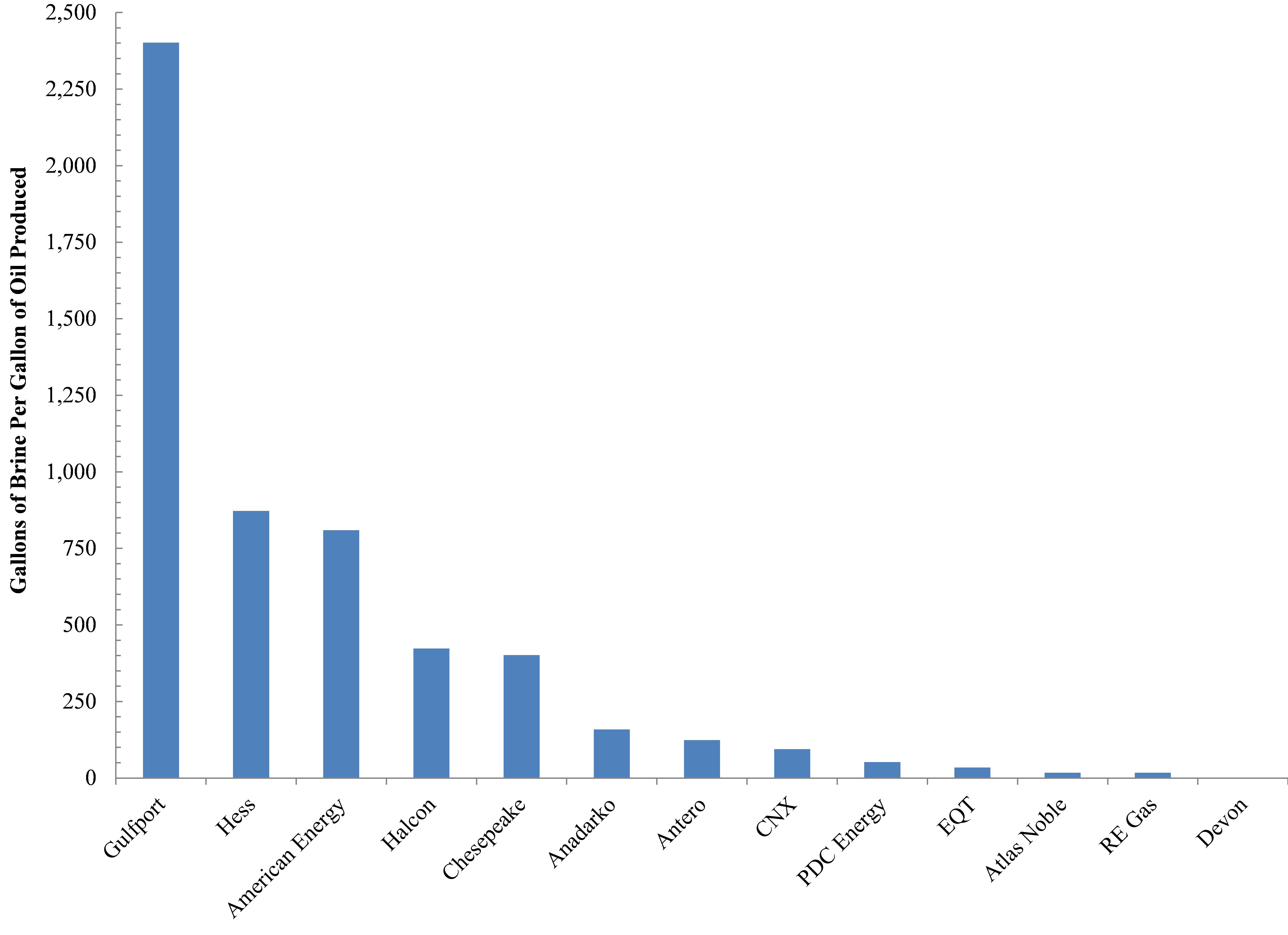
Figure 5. Brine-to-Oil Ratios among Ohio Utica Operators
With respect to the relationship between hydrocarbon and waste generation, we see that no firm can match Oklahoma City-based Gulfport’s inefficiencies with an average of 2,400+ gallons of brine produced per gallon of oil.
American Energy and Hess are not as wasteful, but they are the only other firms generating more than 750 gallons brine waste per unit of oil.
Houston-based Halcon and OH’s primary Utica player Chesapeake Energy are generating slightly more than 400 gallons of brine per gallon of oil.
The remaining firms are generating between 17 (Atlas Noble and RE Gas) and 160 (Anadarko) gallons of brine per unit of oil.
Part II of the Series
In the next part of this series we will look into inter-county differences as they relate to water use, production, and lateral length. Additionally, we will also examine how the OH DNR’s initial Utica projections differ dramatically from the current state of affairs.
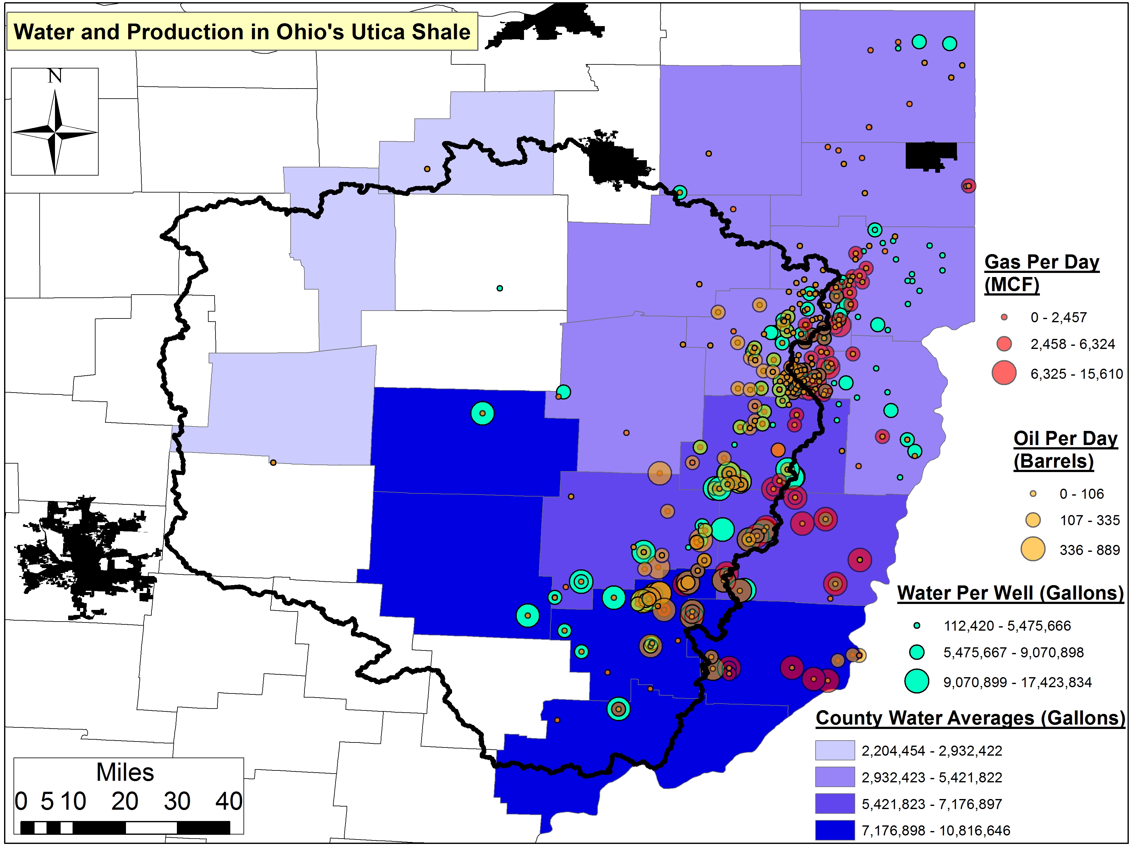
Water and Production in Ohio’s Utica Shale – Water Per Well
https://www.fractracker.org/a5ej20sjfwe/wp-content/uploads/2014/10/Production-Feature.png400900Ted Auch, PhDhttps://www.fractracker.org/a5ej20sjfwe/wp-content/uploads/2025/09/2025-Wordmark-Logo.pngTed Auch, PhD2014-10-24 11:19:272020-07-21 10:34:05The Water-Energy Nexus in Ohio, Part I
Part of the FracTracker Truck Counts Project By Mary Ellen Cassidy, Community Outreach Coordinator, FracTracker Alliance
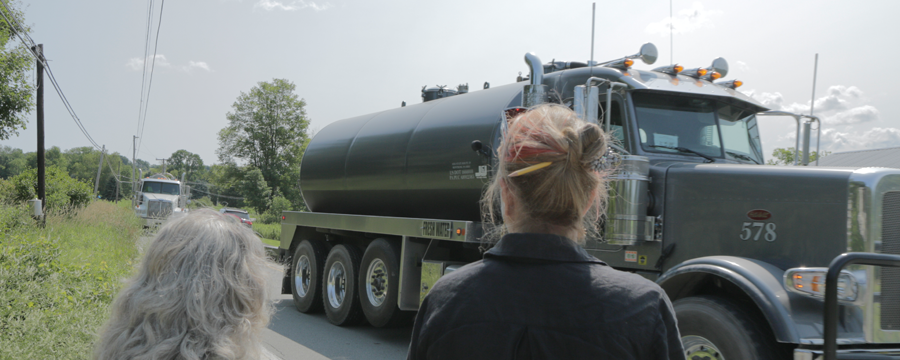
I was recently invited by a community member to visit his home. It sits in a valley that is surrounded by drilling pads, as well as compressors and processing stations. While walking down the road that passes directly in front of his home, several caravans of gas trucks roared past and continued far into the evening. Our discussion about the unexpected barrage of this new invasion of intense truck traffic was frequently interrupted by the noise of the diesel engines passing nearby. Along with the noise, truck headlights pierced through the windows of the home, and dust flew up from the nearby road onto his garden.
There are many stories like this about homes and families impacted by the increased truck traffic associated with fracking-related activities. FracTracker is currently working with some of these communities to document the intensity of gas and oil trucks travelling their roads. In response to these concerns we have a launched a pilot Truck Counts project to provide support, resources, and networking opportunities to communities struggling with high volume gas truck traffic.
Preliminary Results
Volunteers in PA, WV, OH and WI have already started to participate in the project, with some interesting results, photos, observations, and suggestions.
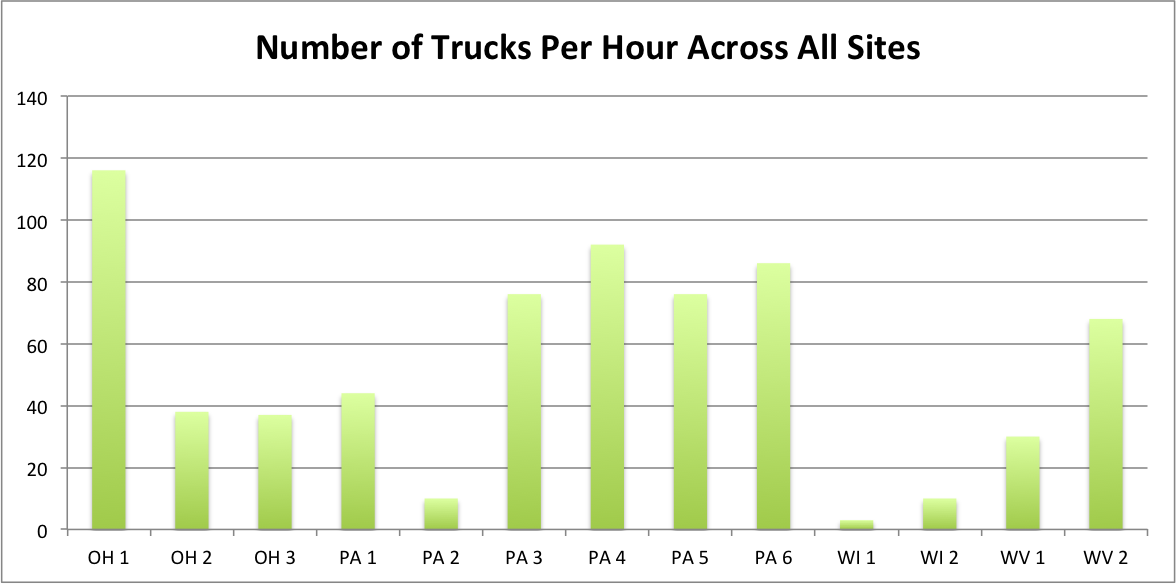
To-date, truck counts have varied significantly, as to be expected. Some of the sites where we chose to count passing trucks were very close to drilling activity, and some were more remote. While developing the counting protocol, we often included large equipment and tanker trucks, as well as gas company personnel vehicles (as indicated by white pickup trucks and company logos on the side). While the data vary, the spikes in truck counts do tell the story of a bigger and broader issue – the influx of heavy equipment during certain stages of drilling can be a significant burden on the local community. In total, we counted 676 trucks over 13 sites The average number of trucks that passed by per hour was 44, with a high of 116 an hour, and a low of 5.
About the Project
FracTracker Truck Counts partners with communities to: help identify issues of concern related to high volume gas truck traffic; collect data, photos, videos and narratives related to gas truck traffic; and analyze and share results through shared database and mapping options.
What motivates volunteers to join us in our Truck Counts program? Community concerns include dust, diesel exhaust, spills, accidents, along with other health and safety issues, as well as the cost and inconvenience of deteriorating road conditions resulting from the increased weights and numbers of vehicles. So, what do we already know about the extent of the damages caused by heavy truck traffic?
Public Safety
Several studies have found that shale gas development is strongly linked to increased traffic accidents and that the increases cannot be attributed only to more trucks and people on the road.
Unlike gas truck traffic issues from past oil and gas booms, this recent shale gas boom impacts traffic and public safety in many different ways. The hydraulic fracturing process requires 2,300 to 4,000 truck trips per well, where older drilling techniques needed one-third to one-half as many trips. Another difference is the speed of development that often far outpaces the capacity of communities to build better roads, bridges, install more traffic signals or hire extra traffic officers. Some experts explain increased truck traffic related accidents by pointing to regulatory loopholes such as federal rules that govern how long truckers can stay on the road being less stringent for drivers in the oil and gas industry. Others note that out of state drivers in charge of large heavy duty loads are not always accustomed to the regional weather patterns or the winding, narrow and hilly country roads that they travel.
An Associated Press analysis of traffic deaths in six drilling states shows that in some counties, fatalities have more than quadrupled since 2004 when most other American roads have become much safer in that period (even with growing populations). Marvin Odum, who runs Royal Dutch Shell’s exploration operations in the Americas, said that deadly crashes are “recognized as one of the key risk areas of the business”. Along with the community, gas truck drivers themselves are at risk. According to a study by the National Institute for Occupational Safety and Health, vehicle crashes are the single biggest cause of fatalities to oil and gas workers. The AP study finds that:
In North Dakota drilling counties, the population has soared 43% over the last decade, while traffic fatalities increased 350%. Roads in those counties were nearly twice as deadly per mile driven than the rest of the state
From 2009-2013-
Traffic fatalities in West Virginia’s most heavily drilled counties…rose 42%. Traffic deaths in the rest of the state declined 8%.
In 21 Texas counties where drilling has recently expanded, deaths/100,000 people are up an average of 18 % while for the rest of Texas, they are down by 20%.
Traffic fatalities in Pennsylvania drilling counties rose 4%, while in the rest of the state they fell 19 %.
New Mexico’s traffic fatalities fell 29%, except in drilling counties, where they only fell 5%.
A separate analysis by Environment America using data from the Upper Great Plans Institute finds that – “While the expanding oil industry in North Dakota has produced many benefits, the expansion has also resulted in an increase in traffic, especially heavy truck traffic. This traffic has contributed to a number of crashes, some of which have resulted in serious injuries and fatalities.” In the Bakken Shale oil region of North Dakota, the number of highway crashes increased by 68% between 2006 and 2010, with the share of crashes involving heavy trucks also increasing over that period.”1
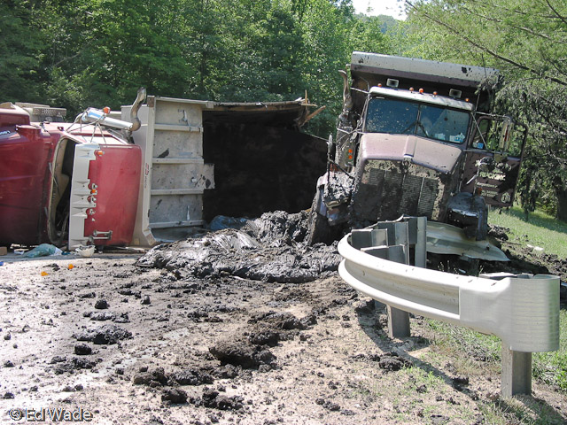
Truck accident and spill in WV. Wetzel County Action Group photo, copyright of Ed Wade, Jr.
Public health concerns do not end with traffic accidents and fatalities. An additional cost of heavy gas truck traffic is the strain it places on emergency service personnel. A 2011 survey by State Impact Pennsylvania in eight counties found that:
Emergency services in heavily drilled counties face a troubling paradox: Even though their population has fallen in recent years, 911 call activity has spiked — by as high as 46 percent, in one case.” Along with the demands placed on emergency responders from the number of increased calls, it also takes extra time to locate the accidents since many calls are coming from transient drivers who “don’t know which road or township they are in.
In Bradford County, a heavily drilled area, increased traffic has delayed the response times of emergency vehicles. According to an article in The Daily Review, firefighters and emergency response teams are delayed due to the increased number of accidents, gas trucks breaking down, and gas trucks running out of fuel (some companies only allow refueling once a night).
Road Deterioration and Regional Costs
Roadway degradation from truck traffic. Wetzel County Action Group photo, copyright of Ed Wade, Jr.
An additional cost often passed on to the impacted communities is infrastructure maintenance. In an article from Business Week, Lynne Irwin, director of Cornell University’s local roads program in Ithaca, New York, states, “Measures to ensure that roads are repaired don’t capture the full cost of damage, potentially leaving taxpayers with the bill.”
This Food and Water Watch Report calculated the financial burden imposed on rural counties by traffic accidents alone, estimating that if the heavy truck accident rate in fracked counties had matched those untouched by the boom, $28 million would have been saved.2
Garrett County is currently struggling with anticipating potential gas traffic and road costs. The Garrett County Shale Gas Advisory Committee uses recent studies from RESI ‘s New York and Pennsylvania data to project gas truck traffic for 6 wells/pad at 22,848 trips/pad and 91,392 total truck trips the first year with increasing numbers for the next 10 years. Like many counties, Garrett County also faces the issue that weights and road use are covered by State, not County code. There is a possibility, however, that the County could determine best “routes” for the trucks. (This is a prime example of the need and benefit for truck counts.)
Although truck companies and contractors pay permit fees, often they are either insufficient to cover costs or are not accessible to impacted counties. The Texas Tribune reports, “The Senate unanimously passed a joint resolution which would ask voters to approve spending $5.7 billion from the state’s Rainy Day Fund, including $2.9 billion for transportation debt. But little, if any, of that money is likely to go toward repairing roads in areas hit hardest by the drilling boom.”
Commenting on the argument that gas companies already pay their fair share for road damages they cause, George Neal posts calculations on the Damascus Citizens for Sustainability website that lead him to conclude that, although “the average truck pays around 27 times the fuel taxes an average car pays… according to the Texas Department of Transportation, they do 8,000 times the damage per mile driven and drive 8 times as far each year.”
The funds needed to fill the gap between the costs of road repairs and the amount actually paid by the oil and gas companies must come from somewhere. According to a draft report from the New York Department of Transportation looking at potential Marcellus Shale development costs, “The annual costs to undertake these transportation projects are estimated to range from $90 to $156 million for State roads and from $121-$222 million for local roads. There is no mechanism in place allowing State and local governments to absorb these additional transportation costs without major impacts to other programs and other municipalities in the State.”
Poor Air Quality
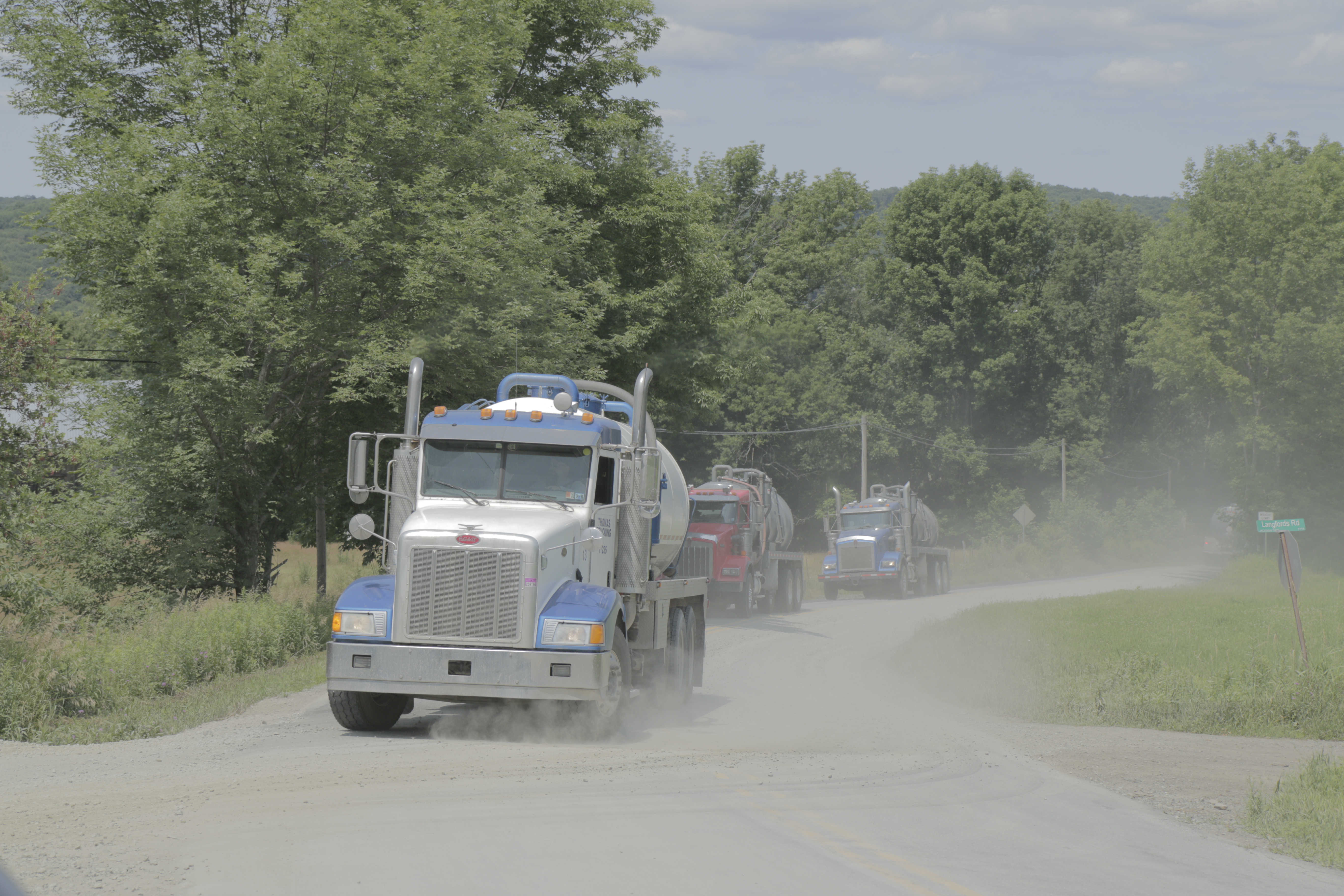
Caravan of trucks. Photo by Savanna Lenker, 2014.
Along with public safety and infrastructure costs, increased truck traffic associated with unconventional oil and gas extraction is found to be a major contributor to public health costs due to elevated ozone and particulate matter levels from increased emissions of heavy truck traffic and the refining and processing activities required.
In addition to ozone and particulate matter in the air, chemicals used for extraction and development also pose a serious risk. A recent study in the journal of Human and Ecological Health Assessment found that 37% of the chemicals used in drilling operations are volatile and could become airborne. Of those chemicals, more than 89% can cause damage to the eyes, skin, sensory, organs, respiratory and gastrointestinal tracts, or the liver, and 81% can cause harm to the brain and nervous system. Because these chemicals can vaporize, they can enter the body not only through inhalation, but also absorption through the skin.
The Union of Concerned Scientists note that air pollution from traffic may be worsened in North Dakota by the use of unpaved roads that incorporate gravel containing a fibrous mineral called erionite, which has properties similar to asbestos. Trucks driving over such gravel roads can release harmful dust plumes into the air, which could present health risks for workers and area residents
To address and solve these problems associated with heavy truck traffic, information is needed to assess both qualitatively and quantitatively the scope of the increased truck traffic and its impacts on communities. Collection and analysis of data, as well as community input, are needed to both understand the scope of the problem and to inform effective solutions.
Joining FracTracker’s Truck Counts
In response to community concerns about the impacts of increased truck traffic in their community, FracTracker has developed the Truck Count project to document the intensity of oil and gas traffic in your region, map heavy traffic locations, and offer networking opportunities for impacted communities.
Participation in FracTracker’s Truck Counts can provide grassroots organizations with a valuable opportunity to collect local data, engage volunteers, and educate stakeholders and the public. The data, pictures and narratives collected can be used to support concerned citizens’ efforts to reroute traffic from schools, playgrounds and other sensitive areas; to inform decision makers, public health researchers, and transportation agencies; to serve as a potential launching point for more detailed, targeted studies on public health and safety along with economic development analyses; to compare costs and benefits of oil and gas energy sources to the cost and benefits of energy conservation, efficiency and renewable energy.
Also, by sharing your community’s counts and stories on FracTracker.org, you serve other communities by increasing the awareness of the impacts of oil and gas truck traffic nationwide.
FracTracker’s Truck Counts provides the following resources to conduct the counts:
information and education on gas and oil truck identification,
data sheets for easy counting, and
tips for selecting safe and accessible counting locations in your community.
We look forward to working with you and supporting your community. If you are interested in working on this important crowdsourcing project with us, please contact:
In addition, a 2013 study from Resources for the Future found that shale gas development is linked to traffic accidents in Pennsylvania with a significant increase in the number of total accidents and accidents involving a heavy truck in counties with a relatively large degree of shale gas development as compared to counties with less (or no) development.
The 2013 Food and Water Watch Report finds similar correlations. Shale gas drilling was associated with higher incidents of traffic accidents in Pennsylvania. This trend was strongest in counties with the highest density of fracking wells. The decrease in the average annual number of total vehicle crashes was 39% larger in unfracked rural counties than in heavily fracked counties. (analysis based on data from US Census Bureau, PA DEP and PennDOT).
In a recent Karnes County, Texas analysis “Traffic accidents and fatalities have skyrocketed in the shale boom areas….with an increases of 1,000% in commercial motor vehicle accidents from 2008-2011.
According to a 2013 Texas Public Threat Safety Report, “In the three Eagle Ford Shale counties where drilling is most active, the number of crashes involving commercial vehicles rose 470 percent between 2009 and 2011. In the 17 counties that make up the Permian Basin, fatal car crashes involving commercial vehicles have nearly tripled from 14 in 2010 to 41 in 2012.
As a result of heavily using of publicly available infrastructure and services, fracking imposes both immediate and long-term costs on taxpayers. An Environment Texas study reveals that, “Trucks required to deliver water to a single fracking well cause as much damage to roads as 3.5 million car journeys, putting massive stress on roadways and bridges not constructed to handle such volumes of heavy traffic. Pennsylvania estimates that repairing roads affected by Marcellus Shale drilling would cost $265 million”.
Researchers from the RAND Corporation and Carnegie Mellon University looked at the design life and reconstruction cost of roadways in the Marcellus Shale formation in Pennsylvania. Their findings in Estimating the Consumptive Use Costs of Shale Natural Gas Extraction on Pennsylvania Roadways, note that local roads are generally designed to support passenger vehicles, not heavy trucks, and that “the useful life of a roadway is directly related to the frequency and weight of truck traffic using the roadway.” The study’s findings include:
“The estimated road-reconstruction costs associated with a single horizontal well range from $13,000 to $23,000. However, Pennsylvania often negotiates with drilling companies to rebuild smaller roads that are visibly damaged, so the researchers’ conservative estimate of uncompensated roadway damage is $5,000 and $10,000 per well.
While the per-well figure of $5,000-$10,000 appears small, the increasingly large number of wells being drilled means that substantial costs fall on the state: “Because there were more than 1,700 horizontal wells drilled [in Pennsylvania] in 2011, the statewide range of consumptive road costs for that year was between $8.5 and $39 million,” costs paid by state transportation authorities, and thus taxpayers.”
The feature photo at the top of the page was taken by Savanna Lenker, 2014.
https://www.fractracker.org/a5ej20sjfwe/wp-content/uploads/2014/09/TruckCounts.png400900FracTracker Alliancehttps://www.fractracker.org/a5ej20sjfwe/wp-content/uploads/2025/09/2025-Wordmark-Logo.pngFracTracker Alliance2014-09-11 15:18:072020-07-21 10:42:44Here They Come Again! The Impacts of Oil and Gas Truck Traffic
Commentary on Shale Gas Operations: First in a Series of Articles
By Bill Hughes, Community Liaison, FracTracker Alliance
Statoil Well Pad Fire: June 28-29, 2014
The early riser residents along Long Ridge Road in Monroe County are among the first in Ohio to see the sun coming up over the West Virginia hills. It rose about 6:00 am on the morning of June 28th. Everyone assumed that this would be a normal Saturday morning. Well, at least as normal as it had been for the better part of two years since the site preparation and drilling started.
For those residents on Long Ridge who were not early risers, the blaring sirens, the smell of acrid smoke, and the presence of fire trucks and other emergency vehicles shortly after 9:00 am must surely have made them wonder if they were in the midst of a nightmare. A quick glance outside toward the Statoil Eisenbarth well pad and they would have seen this view:
Figure 1. View from the southeast, as the fire spread on Sat. June 28th
The image in Fig. 1 would be enough to make most folks feel somewhat panicky and consider evacuating the neighborhood. That is exactly what soon happened – definitely not the start of a normal Saturday morning.
Adjusting to the New Normal
The traffic in the area had been a problem ever since site preparation started on the nearby well pad. The State expected the drillers to keep up the road. Crews also provided lead escort vehicles to help the many big trucks negotiate the narrow road way and to clear the residential traffic. Access to the well site required trucks to climb a two-mile hill up to the ridge top.
Fig. 2. Neighbors’ views of the fire
Until June 28th, most folks had become accustomed to the extra noise, diesel fumes, and congestion and delays that always come with any shale gas well exploration and development in the Marcellus shale gas active area. Most of the neighbors had gotten used to the new normal and reluctantly tolerated it. Even that was about to change, dramatically. As the sun got higher in the eastern sky over WV, around 9:00 AM, suddenly the sky started to turn dark. Very dark. Sirens wailed. Red trucks started a frenzied rush down Long Ridge from all directions. There was a fire on the well pad. Soon it became a very large, all consuming fire. Smoke, fire, bitter fumes, and no one seemed to know yet exactly what had happened, and what was likely to happen soon.
This gas well location, called the Eisenbarth pad, recently changed operators. In January 2013, the well pad property and its existing well and equipment were bought out by Statoil, a company based in Norway. Statoil had since drilled seven more wells, and even more were planned. The original single well was in production. Now in late spring and early summer of 2014 the new wells were to be “fracked.” That means they were ready to be hydraulically fractured, a procedure that follows the completion of the drilling process.
Statoil hired as their fracturing sub-contractor Halliburton. All of the fracturing pump trucks, sand kings, Sand Castles, and control equipment were owned and operated by Halliburton. The fracturing process had been ongoing for some weeks when the fire started. The eastern Ohio neighbors now watched ~$25 million worth of equipment go up in smoke and flames (Fig. 2). The billowing smoke was visible for over 10 miles.
Industrial accidents are not rare in the Ohio Valley
Many of the residents nearby had worked in the coal mining industry, aluminum plants, chemical plants, or the coal fired power plant that were up and down the Ohio River. Many had since retired and had their own industrial accident stories to tell. These were frequently private stories, however, which mostly just their co-workers knew about. In an industrial plant, the common four walls and a roof kept the dangerous processes confined and enabled a trained response to the accidents. The traditional, industrial workplace had well-proven, customized workplace safety standards. Professional maintenance personnel were always nearby. In stark contrast, unconventional gas well pads located in our rural communities are very different. They are put in our hayfields, near our homes, in our pastures and just down the road. You cannot hide a community accident like this.
Sept 2014 Update: Video of the fire, Copyright Ed Wade, Jr.
Print Media Coverage of the Fire
Within days, many newspapers were covering the well pad fire story. The two nearby weekly newspapers, one in Monroe County, Ohio and the other in Wetzel County, West Virginia both had detailed, long articles the following week.
Fig. 3. View from the east as the fire started
The Monroe County Beacon on July 2, 2014 said that the fire spread quickly from the small original fire which was totally surrounded within the tangled complex of equipment and high pressure piping. Early Saturday morning, the first responder would likely have seen a rather small somewhat localized fire as shown in Fig. 2. The photo to the right (Fig. 3) is the view from the east, where the access road is on Long Ridge road. This point is the only access into the Statoil well pad. The view below, showing some still intact tanker trucks in the foreground, is looking west toward the well location. Pay attention to the couple of trucks still visible.
The Monroe County emergency director said it was his understanding that the fire began with a ruptured hydraulic hose. The fluid then ignited on a hot surface. He said, “…by 9:10 AM the fire had spread to other pumps on the location and was spreading rapidly over the well pad.” Emergency responders needed water now, lots of it. There is only one narrow public road to the site at the top of a very long, steep hill and only one narrow entrance to the densely congested equipment on the pad. Many Volunteer Fire Departments from both Ohio and West Virginia responded. A series of tanker trucks began to haul as much water to the site as possible. The combined efforts of all the fire departments were at best able to control or contain but not extinguish the powerful, intensely hot and growing blaze. The Volunteer firemen did all they could. The EMS director and Statoil were very grateful for the service of the Volunteer Fire Departments. There was a major loss of most equipment, but none of the 45-50 workers on site were injured.
Fig. 4. Well pad entrance
The article from the Wetzel Chronicle also praised the coordinated effort of all the many fire departments. At first they attempted to fight the fire, and then prudently focused on just trying to limit the damage and hoping it did not spread to the well heads and off the well pad itself. The New Martinsville fire chief also said that, “… the abundance of chemicals and explosives on the site, made attempts to halt the fire challenging, if not nearly impossible… Numerous plans to attack the fire were thwarted each time by the fires and numerous explosions…” The intense heat ignited anything nearby that was at all combustible. There was not much choice but to let the fire burn out.
Eventually the view at the well pad entrance as seen from the east (Fig. 3) would soon look like the overhead view (Fig. 5). This aerial imagery shows what little remained after the fire was out – just some aluminum scrap melted into the decking is left of the original, white Hydrochloric Acid tanker truck. Everything near it is has almost vaporized.
Figure 5. Post-fire equipment identification
Efforts to Limit the Fire
Fig. 6. Protected white trailer
An excellent example of VFD’s successfully limiting the spread of the fire and controlling the extreme heat can be seen in the photo to the right (Fig. 6). This white storage trailer sure seems to be a most favored, protected, special and valuable container. It was.
It was filled with some particularly dangerous inventory. The first EPA report explains it thus:
A water curtain was maintained, using pump lines on site, to prevent the fire from spreading to a trailer containing 1,100 pounds of SP Breaker (an oxidizer), 200 pounds of soda ash and compressed gas cylinders of oxygen (3-2000 lb.), acetylene (2-2000 lb.), propane (6-20 lb.), among miscellaneous aerosol cans.
Fig. 7. Post-fire pad layout
Yes, this trailer got special treatment, as it should. It contained some hazardous material. It was also at the far southwest corner of the well pad with minimal combustibles near it. That was also the closest corner to the nearby holding pond, which early on might have held fresh water. Now the holding pond is surely very contaminated from flowback and runoff.
The trailer location can be seen in the picture to the right in the red box (Fig. 7), which also shows the complete well pad and surrounding area. However, in comparison to the one white storage trailer, the remainder of the well pad did not fare so well. It was all toast, and very burned toast at that.
Columbus Dispatch and the Fish Kill
Besides the two local newspapers, and Wheeling Jesuit researchers, the Columbus Dispatch also covered the story and provided more details on the 3- to 5-mile long fish kill in the stream below the well pad. Additional facts were added by the two EPA reports:
Those reports list in some detail many of the chemicals, explosives, and radiological components on the well pad. Reader note: Get out your chemical dictionary, or fire up your Google search. A few excerpts from the first EPA report are provided below.
…Materials present on the Pad included but was not limited to: diesel fuel, hydraulic oil, motor oil, hydrochloric acid, cesium-137 sources, hydrotreated light petroleum distillates, terpenes, terpenoids, isoproponal, ethylene glycol, paraffinic solvents, sodium persulfate, tributyl tetradecyl phosphonium chloride and proprietary components… The fire and explosion that occurred on the Eisenbarth Well Pad involved more than 25,000 gallons of various products that were staged and/or in use on the site… uncontained run-off was exiting the site and entering an unnamed tributary of Opossum Creek to the south and west and flowback water from the Eisenbarth Well #7 was spilling onto the well pad.
Reader Warning: If you found the above list overly alarming, you might choose to skip the next equally disturbing list. Especially since you now know that this all eventually flowed into our Ohio River.
The EPA report continues with more specific chemical products involved in the fire:
Initial reports identified the following products were involved and lost in the fire: ~250 gallons of hydrochloric acid (28%), ~7,040 gallons of GasPerm 1000 (terpenes, terpenoids, isopropanol, citrus extract, proprietary components), ~330 gallons of LCA-1 (paraffinic solvents), ~ 1900 gallons of LGC-36 UC (hydrotreated light petroleum distillate, guar gum), ~1000 gallons of BC-140 (monoethanolamine borate, ethylene glycol), ~3300 gallons of BE-9 (tributyl tetradecyl phosphonium chloride), ~30,000 gallons of WG-36 (polysaccharide gel), ~1,000 gallons of FR-66 (hydrotreated light petroleum distillate), ~9000 gallons of diesel fuel, ~300 gallons of motor and hydraulic oil.
Even more details of the incident and the on-site chemicals are given in the required Statoil 30-day report (PDF).
The EPA reports detail the “sheet” flow of unrestricted contaminated liquids off of the well pad during and after the fire. They refer to the west and south sides. The below Google Earth-based map (Fig. 8) shows the approximate flow from the well pad. The two unnamed tributaries join to form Opossum Creek, which then flows into the Ohio River four miles away.
Figure 8. Map showing path of unrestricted flow off of the Statoil well pad due to a lack of berm
After describing some of the known chemicals on the well pad, the EPA report discusses the construction of a new berm, and where the liquid components flowed. Below is a selection of many excerpts strung together, from many days, taken directly from the EPA reports:
…unknown quantities of products on the well pad left the Site and entered an unnamed tributary of Opossum Creek that ultimately discharges to the Ohio River. Runoff left the pad at various locations via sheet flow….Initial inspections in the early hours of June 29, 2014 of Opossum Creek approximately 3.5 miles downstream of the site identified dead fish in the creek…. Equipment was mobilized to begin constructing an earthen berm to contain runoff and to flood the pad to extinguish remaining fires…. Once fires were extinguished, construction of a berm near the pad was begun to contain spilled liquids and future runoff from the well pad… Statoil continued construction of the containment berm currently 80% complete. (6-30-14)… Assessment of chemicals remaining on the well pad was completed. The earthen berm around the pad was completed, (7-2-14)… ODNR Division of Wildlife completed their in stream assessment of the fish kill and reported an estimated 70,000 dead fish from an approximately 5 mile stretch extending from the unnamed tributary just west of the Eisenbarth Well Pad to Opossum Creek just before its confluence with the Ohio River… Fish collection was completed. In total, 11,116 dead fish were collected (20 different species), 3,519 crustaceans, 7 frogs and 20 salamanders.
The overall conclusion is clear. Large quantities of various chemicals, mixed with very large amounts of already contaminated water, when flooding a well pad that had no berms around it, resulted in a significant fish kill over several miles. After the fire Statoil then constructed a berm around the well pad. If there had been a pre-existing berm – just 12 inches high and level – around the well pad, it could have held over 600,000 gallons of runoff. That amount is twice the estimated quantity of water used to fight the fire. (Note: my old 35 HP farm tractor and a single bottom plow can provide a 12-inch high mound of dirt in one pass.)
The significance for safe, potable drinking water, is that all the chemicals and petroleum products on the well pad either burned and went up in a toxic plume of black smoke, or were released in liquid form down into the well pad or flowed off of it. Since the original liner on the well pad also completely burned and there was no overall berm on the well pad, there was nothing to restrict the flow of polluted liquid. Therefore, it all seeped into the ground and/or ran off of the pad with the 300,000 gallons of water that was estimated to have been sprayed onto the burning equipment fire.
Follow Up Questions
Since this fire happened over 6 weeks ago, there have been many opportunities for nearby citizens and neighbors to meet and discuss their many concerns. Many of the question have revolved around the overall lack of information about the process of shale gas fracturing, the equipment used, and the degree of risk that it all may present to our communities. These communities include the nearby residents, the travelling public, and all of the first responders. Unless someone has a well pad on or near their property and they are able to actively follow the process, it is usually difficult to find out the details of a specific gas operation. (We have even known of operators that have told landowners to get off of their own property both during drilling and fracturing operations and afterwards.)
Questions that follow incidents like this one typically look like this:
Why was there no perimeter berm?
Why could the fire not be put out quickly and easily? What all was lost? What did this site look like in the beginning?
Why was there so much equipment onsite? Is this typical? What is it all called and how is it used?
1. Lack of Berm
The first and somewhat unanswered question concerns the absence of a simple containment berm around the completed well pad. Statoil must not have thought one would be very helpful, and/or the State of Ohio must not require them.
However, I had raised concern over this very topic more than a year ago from WV. In response, I received a letter in September 2013 from Statoil North America to the WVDEP. It provides some insight into Statoil thinking. Based on my interpretation of that letter, the official position of Statoil last year was that berms around the well pad do not help and are not needed. Given the recent fire, perhaps that position has changed. All we know for sure now is that at least their Eisenbarth well pad now does have a complete perimeter berm. We now have empirical proof, if any was ever needed, that in the presence of spills the absence of berms makes for greater and more expensive downstream problems.
2. An Obstinate Fire
Setting aside the berm problem, I will attempt to address the next set of questions: Why could the fire not be put out quickly and easily? What all was lost ? What did this site look like in the beginning?
The simplest way to start on such questions is to look at other hydraulic fracturing sites to identify what is there and why, and then to compare those with the charred remains on the Statoil Eisenbarth well pad in Monroe County. Since Statoil’s contractor was Halliburton, it would help to look at their equipment when in process elsewhere. In Figure 9 below is a clean, bright red and grey Halliburton fracking fleet.
Figure 9. Example of Halliburton fracking fleet
It needs to be stated up front that I consider Halliburton to be among one of the more reputable, experienced, and dependable fracturing companies. We have seen way worse here in Wetzel County over the past seven years. Halliburton has good equipment and well-trained, safety-conscious employees. It seems to be a well-run operation. If so, then how did this massive fire happen? It simply seems that it is the nature of the beast; there are many inherent dangers to such operations. Plus there is an enormous amount of equipment on site, close coupled and stuffed into a small amount of real estate. Not to mention, the whole setup is temporary – with a lot of fuel and ignition sources. Therefore, many of the available engineered-in safeguards that would normally be installed in an industrial, fixed, permanent location, just cannot be incorporated on my neighbor’s hay field, creek bottom, or farmland.
The whole process has many risks, and many of them cannot be eliminated, just minimized. I do not think that anyone could have predicted a weak hydraulic hose. Some accidents are just that — unpreventable accidents. This is why we need to be very careful with how close we allow these sites in residential areas.
3. Serious Equipment
In Figure 10 below is a wide-angle composite photo of a Halliburton fracturing project in process. Given the shallow angle viewpoint, not all equipment is visible or numbered. The photo is still very representative of frac sites in general and equivalent to what can be seen in the scorched remains on the Statoil Eisenbarth site. The major qualification on the fracturing pumps above and the ones below, is that they are a newer generation of Halliburton dual fuel pumps. They can run on natural gas.
Figure 10. Halliburton fracturing project in process
Just about everything seen in the above bright red and grey hardware can be seen in Figure 11’s charred leftovers on the Statoil site from July 5, 2014 below (six days after the fire). It is also all Halliburton equipment. The quantities and arrangement are different, but the equipment and process are the same. The numbers on the provided legend or chart should help identify the specific pieces of equipment. The newly constructed containment berm is also clearly visible here.
Figure 11. Statoil site post-fire equipment identification
The above or a similar photo has been seen by many neighbors both in OH and WV. Hardly anyone can recognize what they are looking at. Even those people who are somewhat familiar with general hydraulic fracturing operations are puzzled. Nothing is obvious when viewing charred remains of burned iron, steel, and melted aluminum. All tires (over 400 of them) have been burned off the rims. Every bit of rubber, foam, composites, plastics and fiberglass truck cabs has been consumed – which is what made the black plume of smoke potentially so dangerous.
Fig. 12. 16 fracturing pumps
Fig. 13. 18-wheeler
What might not be so obvious is why the fire could not be extinguished.
If we look at a close-up of a small section of the well pad (Fig. 12) it is easy to see how crowded the well pad is during fracturing. The 16 fracturing pumps are all the size of a full-length 18-wheel tractor trailer (Fig. 13). Note the three fuel tanks.
The fire began between the blender-mixer trucks and the 16 hydraulic fracturing pumps. The blenders were between the fracturing pumps and the sand kings. Halliburton always keeps fire extinguishers available at every truck. They are put on the ground in front of every pump truck. Everyone knows where to find them. However, on any fracking project that location is also the most congested area. The fracturing pumps are usually parked no more than two feet apart. It is just enough room for an operator or maintenance fellow to get between them. With high pressure fluid spraying and the fire already started and now spreading, there is precious little room to maneuver or to work. It is a plumbing nightmare with the dozens of high pressure pipes connecting all the pumps together and then to a manifold. In those conditions, in the face of multiple fuel sources, then the many small explosions, prudence and self-preservation dictates a swift retreat.
To their credit, Halliburton employees knew when to retreat. No one was injured. We just burned up some trucks (and killed some fish). All the employees and all the first responders were able to go home safely, uninjured, to their families and friends. They survived a very dangerous situation to come back again in the service of their employer or their community. We wish them well.
Some Observations and Conclusions
The hydraulic fracturing process is dangerous, even when done properly.
Environmental and employee safeguards must be in place because “accidents will happen.”
Setbacks from personal farm and residential buildings must be great enough to protect all.
Setbacks from streams and creeks and rivers must be taken very seriously, especially when private or municipal water supply systems are downstream.
Our communities must know what all chemicals are being used so that correct lab protocols are established ahead of time to test for contamination.
This now ends this first article addressing the Statoil Fire, its burned fracturing equipment, and the resulting water contamination. Later, I will show many examples of the quantity of equipment used on fracturing sites and why it is there. You patient readers thought this would never end. You now know more about Statoil, well pad fires, and fracturing hardware than you ever wanted to know. We will soon address the more generic questions of fracturing equipment.
https://www.fractracker.org/a5ej20sjfwe/wp-content/uploads/2014/09/StatoilBlog.png400900FracTracker Alliancehttps://www.fractracker.org/a5ej20sjfwe/wp-content/uploads/2025/09/2025-Wordmark-Logo.pngFracTracker Alliance2014-09-08 09:30:582020-07-21 10:42:43In-depth Review of the Statoil Well Pad Fire
By Bill Hughes, Community Liaison, FracTracker Alliance
Monroe County on the eastern border of the State of Ohio and Wetzel County in West Virginia are very much neighbors. They literally share a very deep connection, at least geologically and physically, as they are separated by a very long, deep, 1000-foot wide valley, filled by the Ohio River. A bridge connects the surface land and its residents.
But if you literally dig a little deeper, actually a lot deeper (as in 7,000 feet down), we are seamlessly joined by the Marcellus shale layer. Below this layer, we are joined by other black shale formations where the natural gas and some of its unwelcome neighbors live.
I live in Wetzel County. From where I am sitting I am surrounded by multiple shale gas operations – and have been for over seven years. I have Chesapeake to the north; EQT to the southeast; Stone Energy to the west; Statoil to the east; and HG Energy to the south. They all are primarily extracting gas from the Marcellus formation, but just a few miles to the north of here is a Utica formation well pad (situated below the Marcellus Shale layer). It is being fracked as I write this article.
Externalizing Business Costs
Setting aside the different political and regulatory differences that might exist when comparing WV & OH, the terrain, topography, and cultural history are very similar. The impact of shale gas extraction in a rural community seems to be the same everywhere it is happening, as well. We have all had traffic congestion, road accidents, problems with air and water quality, and waste disposal challenges. All of the drilling companies use fresh water from the Ohio River or its tributaries. WV gas producers take much of their brine and flowback fluids to injections wells in OH for disposal. The grateful OH drillers truck their waste products to our landfills here in Wetzel County and the operators seem pleased with the arrangement. Externalizing costs to our communities seems to be an accepted and tolerated business model.
About Statoil
Statoil is a large natural gas producer from Norway. They have wells both here in Wetzel, WV and in Monroe County, OH. On June 28 and 29 of 2014, a massive fire burned out of control on a Statoil well pad called Eisenbarth in Monroe County (map below), during a routine hydraulic fracturing operation. The size, impact, and cause of the Statoil Eisenbarth fire deserve a lot of attention. Since I have Statoil well pads near me, I am somewhat concerned. Therefore, I will be writing about this specific fire and some of the implications for all of us.
A Series of Incident Articles
This photo essay will be presented in two sections. The first will describe the fire along with some of the details and published reports. The second part will use the photos and information to help us all better understand what is meant when we simply make comments on “fracking.” Additionally, I will show which components are commonly present during the hydraulic fracturing process. Explore the in-depth look at this incident.
Location of the Statoil Eisenbarth fire that occurred in June 2014. Click to explore our Ohio Shale Viewer.
https://www.fractracker.org/a5ej20sjfwe/wp-content/uploads/2014/09/StatoilIntroBlog.png400900FracTracker Alliancehttps://www.fractracker.org/a5ej20sjfwe/wp-content/uploads/2025/09/2025-Wordmark-Logo.pngFracTracker Alliance2014-08-29 09:05:482020-07-21 10:42:43Statoil Eisenbarth Well Pad Fire – An Introduction