The majority of FracTracker’s posts are generally considered articles. These may include analysis around data, embedded maps, summaries of partner collaborations, highlights of a publication or project, guest posts, etc.
The Atlantic Sunrise Project or Central Penn Line is a natural gas pipeline Williams Companies has proposed for construction through eight counties of Central Pennsylvania. Williams intends to connect the Atlantic Sunrise to their two Transco pipelines, which extend from the northeast to the Gulf of Mexico. FracTracker discussed and mapped this controversial project as part of a blog entry in June of 2014; since then, the Atlantic Sunrise Project has been, and continues to be, a focus of unprecedented opposition. While supporters of the pipeline stress how it may enhance energy independence, economic growth, and job opportunities, opponents cite Williams’ poor safety records, their threats of eminent domain, and environmental hazards. This article provides details and maps pertaining to these threats and concerns.
Atlantic Sunrise: Project Overview
The Atlantic Sunrise Project would add 183 miles of new pipeline through the construction of the Central Penn Line North and the Central Penn Line South. The proposed Central Penn Line North (CPLN) begins in Susquehanna County, continues through Wyoming and Luzerne counties, and meets with the Transco Pipeline in Columbia County. With a 30 inch in diameter, it would allow for a maximum pressure of 1,480 psi (pounds per square inch). The proposed Central Penn Line South (CPLS) begins at the Transco Pipeline in Columbia County, and continues through Northumberland, Schuylkill, and Lebanon counties, ending in Lancaster. It would be 42 inches in diameter with a maximum pressure of 1,480 psi. The Atlantic Sunrise project also involves the construction of two new compressor stations, one in Clinton Township, Wyoming County, and the other in Orange Township, Columbia County. Finally, to accommodate the daily 1.7 million dekatherms (1 dekatherm equals 1,000 cubic feet of gas or slightly more than 1 million BTUs in energy) of additional natural gas that would flow through the system, the project proposes the expansion of 10 existing compressor stations along the Transco Pipeline in Pennsylvania, Maryland, Virginia, and North Carolina. Although the Atlantic Sunrise Pipeline would be entirely within Pennsylvania, it is permitted and regulated by the Federal Energy Regulatory Committee (FERC) because through its connection to the Transco Pipeline, it transports natural gas over state lines.
Updated Central Penn Pipeline Route
On March 31, 2015, Williams filed their formal application to FERC docket #CP15-138. Along with the formal application came changes to the pre-filing route of the pipeline that was submitted in the spring of 2014. The route of the Central Penn Line North has been modified since then by 21%, while the Central Penn Line South has been rerouted by 57%.
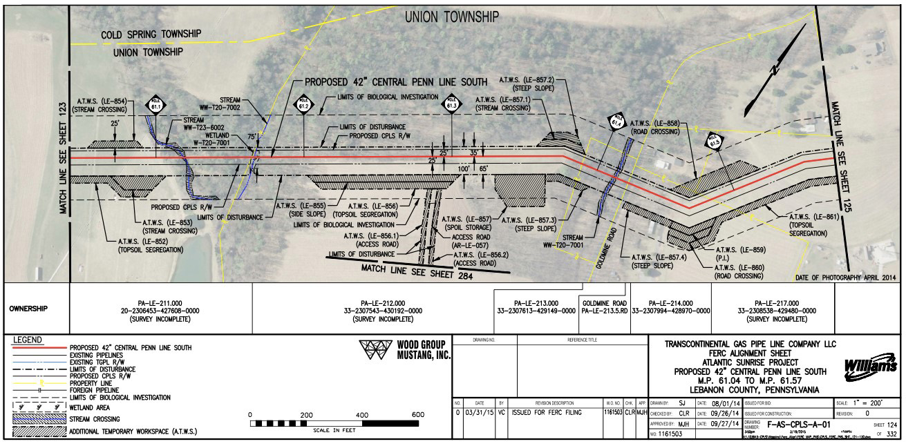
Williams’ application comprised of hundreds of attached documents, including pipeline alignment sheets for the entire route. Here is one example:
These alignment sheets show the extent of William’s biological investigation, the limits of disturbance, the occurrence of stream and wetland crossings, and any road or foreign pipeline crossings. Absent from the alignment sheets, however, is the area around the right-of-way that will be endangered by the presence of the pipeline. This is colloquially known as the “burn zone” or “hazard zone”.
What are “Hazard Zones”?
A natural gas pipeline moves flammable gas under extreme pressure, creating a risk of pipeline rupture and potential explosion. The “potential impact radius” or “hazard zone” is the approximate area within which there will be immediate damage in the case of an explosion. Should this occur, everything within the hazard zone would be incinerated and there would be virtually no chance of escape or survival. Based on pipeline diameter and pressure, the hazard zone can be calculated using the formula: potential impact radius = 0.69 * pipeline diameter * (√max pressure ).
Based on this formula, the hazard zone for the Central Penn Line North, with its diameter of 30 inches and maximum pressure of 1,480 psi, is approximately 796 feet (243 meters) on either side of the pipeline. The hazard zone for Central Penn Line South, with its diameter of 42 inches and maximum pressure of 1480 psi, is 1,115 feet (340 meters) on either side.
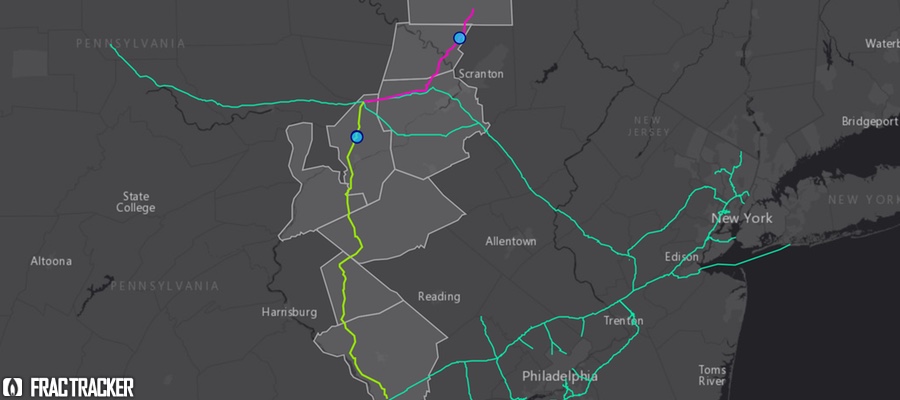
Many residents are unaware that their homes, workplaces, and schools are located within the hazard zone of the proposed Atlantic Sunrise Pipeline. Williams does not inform the public about this risk, primarily communicating with landowners along the right-of-way. The interactive, zoomable map (below) of the currently proposed route of the Atlantic Sunrise, Central Penn North and South pipelines depicts the pipeline right-of-way, as well as the hazard zones. The pipeline route was digitized using the alignments sheets included in Williams’ documents submitted to FERC. You can use this map to search home, work, and school addresses to see how the pipeline will affect residents’ lives and the lives of their communities.
Click in the upper right-hand corner of the map to expand to full-screen view, with a map legend.
Affected Communities
Landowners & Eminent Domain
Landowners along the right-of-way are among the most directly and most negatively impacted by the Atlantic Sunrise Pipeline, and other similar projects. Typically, people first become aware that a pipeline is intended to pass through their property when they receive a notice in the mail. Landowners faced with this news are on their own to negotiate with the company, navigate the FERC permitting and public comment process, and access unbiased and pertinent information. They face on-going stress, experiencing pressure from Williams to sign easement agreements, concern about the effects of construction on their property, and fear of living near explosive infrastructure. They must also consider costs of legal representation, decreases in property value, and limited options for mortgage and refinancing.
Sometimes, landowners in a pipeline’s right-of-way choose to not allow the company onto their property to conduct a survey. Landowners may also refuse to negotiate an agreement with the pipeline company. In response, the pipeline company can threaten to seize the property through the power of eminent domain, the federal power allowing private property to be taken if it is for the “public use.”
The law of eminent domain states that landowners whose properties are condemned must be fairly compensated for their loss. However, most landowners feel that in order to be fairly compensated by the company, they must hire their own land appraiser and attorney. This decision can be costly, however, and may not be an option for many people. The legitimacy of Williams’ intent to use eminent domain is contested by opponents of the project, who cite how “public use” of the property provides no positive local impacts. The Atlantic Sunrise Pipeline is intended to transport gas out of Pennsylvania through the Transco, so the landowners in its path will not benefit from it at all. Further, it connects to a network of pipelines leading to current export terminals in the Gulf of Mexico, as well as controversial planned export facilities like Cove Point, MD .
Throughout Pennsylvania, communities have responded to the expansion of pipelines, and to the threats of large companies like Williams. The need for landowner support has been addressed by organizations such as the Shalefield Organizing Committee, Energy Justice Network, the Clean Air Council, the Gas Drilling Awareness Coalition, and We Are Lancaster County. These organizations have worked to provide information, increase public awareness, engage with FERC, and develop resistance to the exploitation of Pennsylvania’s resources and residents. Director Scott Cannon of the Gas Drilling Awareness Coalition has documented firsthand the impacts of unconventional drilling in Pennsylvania through a short film series called the Marcellus Shale Reality Tour. The most recent in the series relates the stories of two landowners impacted by the Atlantic Sunrise Pipeline in the short film Atlantic Sunrise Surprise.
Environmental Review
Theoretically, environmental review of this proposed pipeline would be extensive. Primary decision-making on the future of the Atlantic Sunrise rests with FERC. Due to the National Environmental Policy Act of 1969 (NEPA), all projects overseen by federal agencies are required to prepare environmental assessments (EAs) or environmental impact assessments (EIAs). Because FERC regulates interstate pipelines, EA’s or EIA’s are required in their approval process. These assessments are conducted to accurately assess the environmental impacts of projects and to ensure that the proposals comply with federal environmental laws such as the Endangered Species Act, and the Clean Air and Water Acts. On the state level, the Pennsylvania Department of Environmental Protection (PA DEP) issues permits for wetlands and waterways crossings and for compressor stations on regional basis.
Core Habitats, Supporting Landscapes
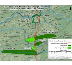
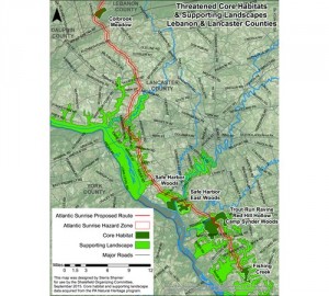
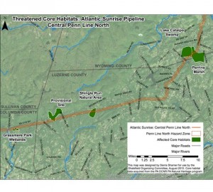
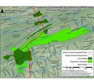
The route of the Atlantic Sunrise Pipeline will disturb numerous areas of ecological importance, including many documented in the County Natural Heritage Inventory (CNHI). The PA Department of Conservation and Natural Resources conducted the inventory to be used as a planning, economic, and infrastructural development tool, intending to avoid the destruction of habitats and species of concern. The following four maps show the CNHI landscapes affected by the current route of the Atlantic Sunrise pipeline (Figures 1-4).
Figure 1. Columbia & Northumberland counties
Figure 2. Lebanon & Lancaster counties
Figure 3. Threatened Core Habitats
Figure 4. Schuyklill & Lebanon counties
The proposed pipeline would disrupt core habitats, supporting landscapes, and provisional species-of-concern sites. According to the Natural Heritage Inventory report, core habitats “contain plant or animal species of state or federal concern, exemplary natural communities, or exceptional native diversity.” The inventory notes that the species in these habitats will be significantly impacted by disturbance activities. Supporting landscapes are defined as areas that “maintain vital ecological processes or habitat for sensitive natural features.” Finally, the provisional species of concern sites are regions where species have been identified outside of core habitat and are in the process of being evaluated. The Atlantic Sunrise intersects 16 core habitats, 12 supporting landscapes, and 6 provisional sites.
Active Mine Fires
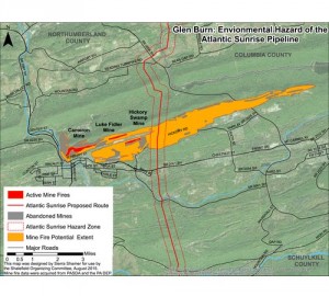
Figure 5. Glen Burn Mine Fires
The current route of the Atlantic Sunrise intersects the Cameron/Glen Burn Colliery, considered to be the largest man-made mountain in the world and composed entirely of waste coal. This site also includes a network of abandoned mines, three of which are actively burning (Figure 5).
The pipeline right-of-way is roughly a half-mile from the closest burning mine, Hickory Swamp. These mine fire data were sourced from a 1988 report by GAI Consulting Inc. The time frame for the spread of the mine fires is unknown, and dependent on environmental factors. Mine subsidence — when voids in the earth created by mines cause the surface of the earth to collapse — is another issue of concern. Routing the pipeline through this unstable area adds to the risk of constructing the pipeline through the Glen Burn region.
Looking Ahead
The Atlantic Sunrise Project has received an unprecedented level of resistance that continues to grow as awareness and information about the threats and hazards develops. While Williams, FERC, and the PA DEP negotiate applications and permits, work is also being done by many non-profit, research, and grassroots organizations to investigate the environmental, cultural, and social costs of this pipeline. We will follow up with more information about this project as it becomes available.
This article was written by Sierra Shamer, an environmental mapper and activist. Sierra is a member of the Shalefield Organizing Committee and holds two degrees from the University of Maryland, Baltimore County: a B.A. in environmental studies and an M.S. in geography and environmental systems.
https://www.fractracker.org/a5ej20sjfwe/wp-content/uploads/2015/10/Atlantic-Shamer-Feature.jpg400900Guest Authorhttps://www.fractracker.org/a5ej20sjfwe/wp-content/uploads/2025/09/2025-Wordmark-Logo.pngGuest Author2015-10-07 09:31:152020-03-12 17:39:30Maps of Updated Central Penn Pipeline Emphasize Threats to Residents and Environment
Oil, Gas, and Brine Oh My! By Ted Auch, Great Lakes Program Coordinator, FracTracker Alliance
It was just three years ago that the Ohio Geological Survey (OGS) and Department of Natural Resources (DNR) were proposing – and expanding – their bullish stance on the potential Utica Shale oil and gas production “play.” Back in April 2012 both agencies continue[d] to redraw their best guess, although as the Ohio Geological Survey’s Chief Larry Wickstrom cautioned, “It doesn’t mean anywhere you go in the core area that you will have a really successful well.”
What we found is that the OGS projections have not held up to their substantial claims. And here is why…
Background
The Geological Survey eventually parsed the Utica play into pieces:
a large oil component encompassing much of the central part of the state,
natural gas liquids from Ashtabula on the Pennsylvania border southwest to Muskingum, Guernsey, and Noble Counties, and
natural gas counties, primarily, along the Ohio River from Columbiana on the Pennsylvania-West Virginia border to Washington County in the Southeast quarter of the state.
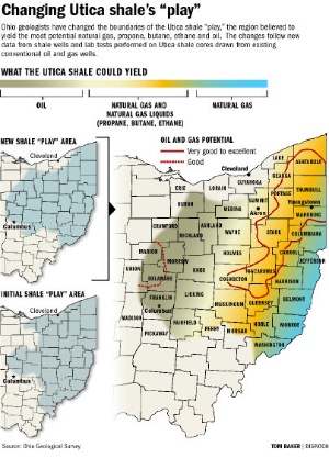
Columbus Dispatch Utica Shale “play” map
Fast forward to the first quarter of 2015 and we have a very healthy dataset to begin to model and validate/refute these projections. Back in 2009 Wickstrom & Co. only had 53 Utica Shale laterals, while today Ohio is host to 962 laterals from which to draw our conclusions. The preponderance of producing wells are operated by Chesapeake (463), Gulfport (118), Antero Resources (62), Eclipse Resources (41), American Energy Utica (36), Consol (35), and R.E. Gas Development (34), with an additional 13 LLCs and 10 publicly traded companies accounting for the remaining 173 producing laterals. A further difference between the following analysis and the OGS one is that we looked at total production and how much oil and gas was produced on a per-day basis.
Analysis
Using an interpolative geostatistical technique known as Empirical Bayesian Kriging and the 962 lateral dataset, we modeled total and per day oil, gas, and brine production for Ohio’s Utica Shale between 2011 and Q1-2015 to determine if the aforementioned map redrawing holds up, is out-of-date, and/or is overly optimistic as is generally the case with initial O&G “moving target” projections.
Days of Activity & Brine Production
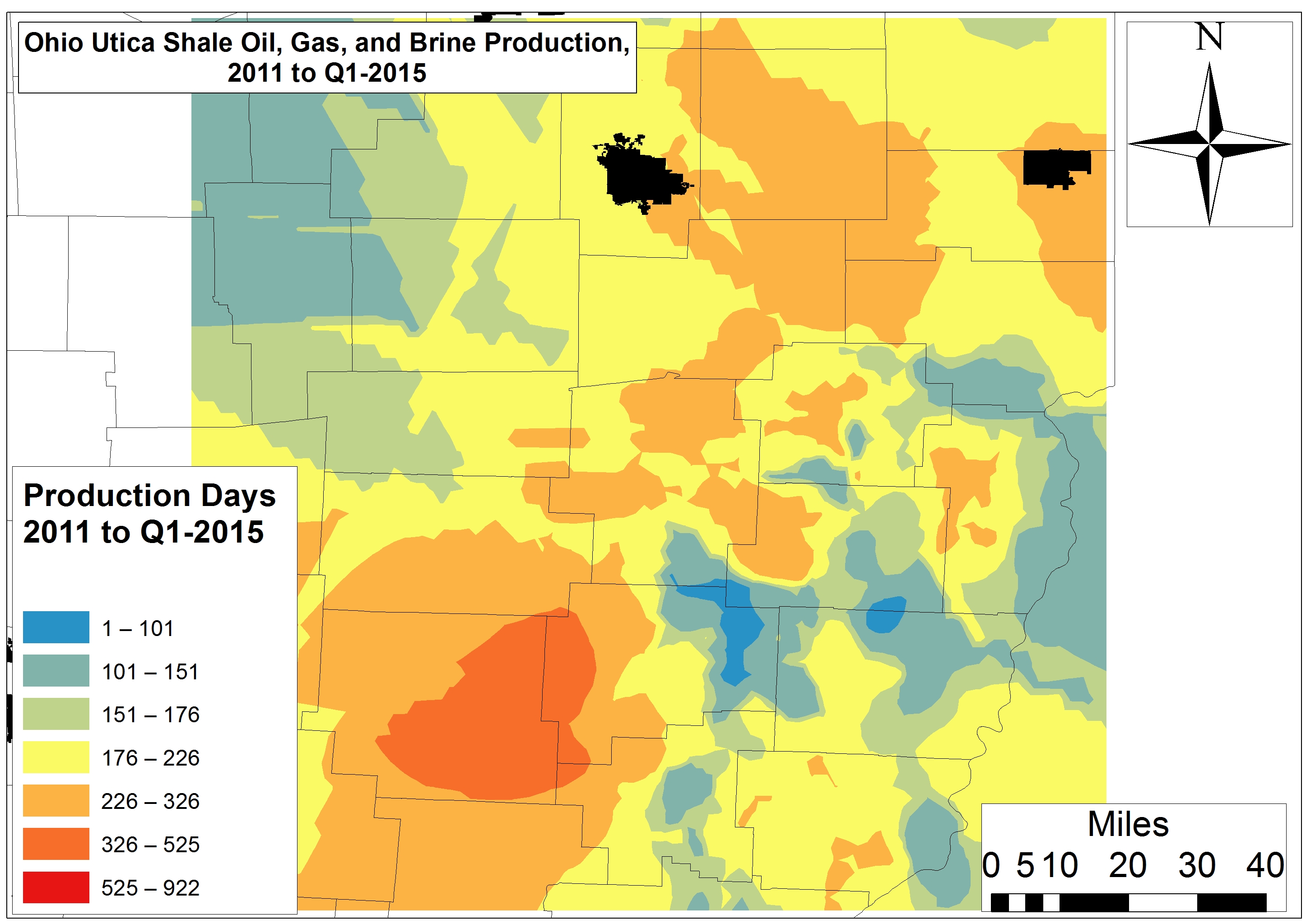
The most active regions of the Utica Shale for well pad activity has been much of Muskingum County and its border with Guernsey and Noble counties; laterals are in production every 1 in 2.1-3.4 days. Conversely, the least active wells have been drilled along the Harrison-Belmont border and the intersection between Harrison, Tuscarawas, and Guernsey counties.
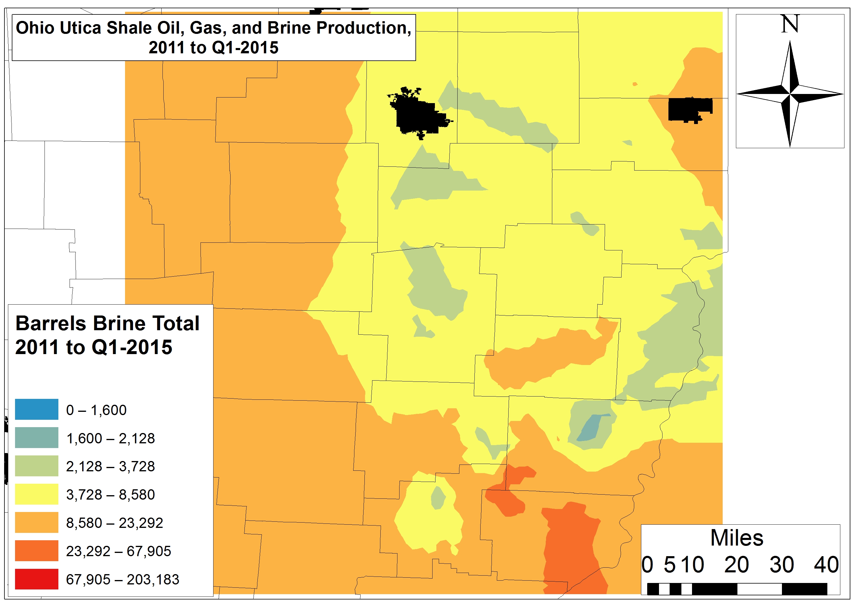
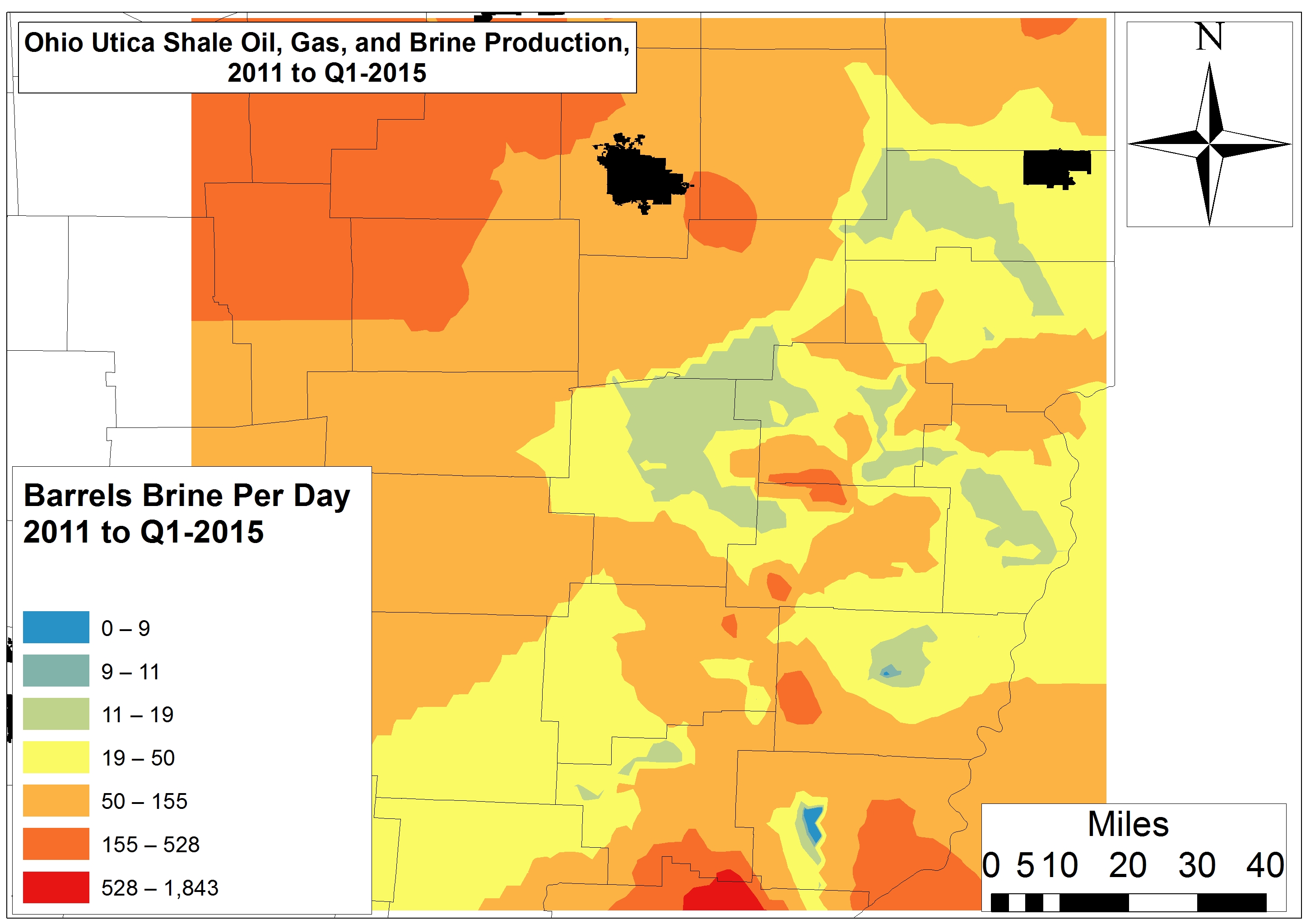
Brine is a form of liquid drilling waste characterized by high salt loads and total dissolved solids. The laterals that have produced the most brine to date are located in a large section of Monroe County and at the intersection of Belmont, Monroe, and Noble counties, with total brine production amounting to 23,292 barrels or 734,000-978,000 gallons (Fig. 1).
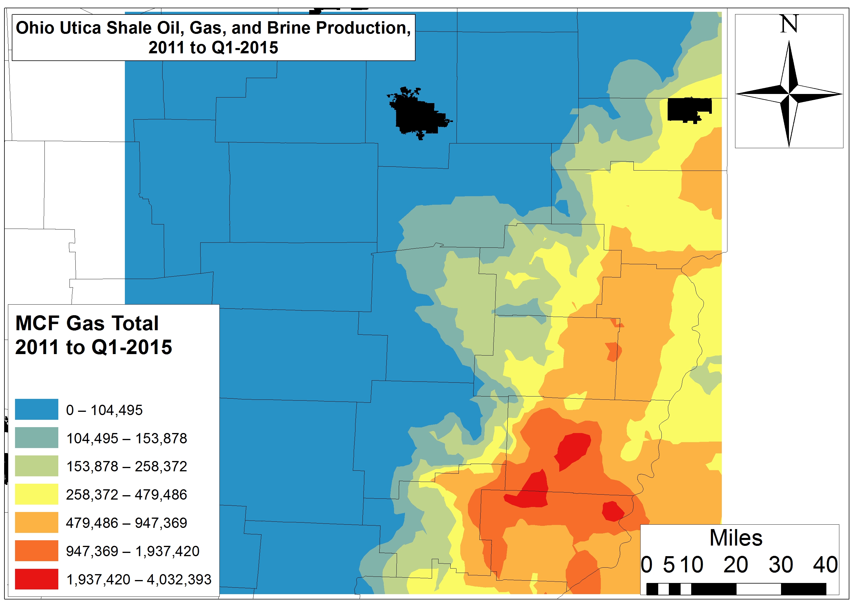
Figure 1. Total Ohio Utica Shale Oil, Gas, and Brine Production 2011 to Q1-2015
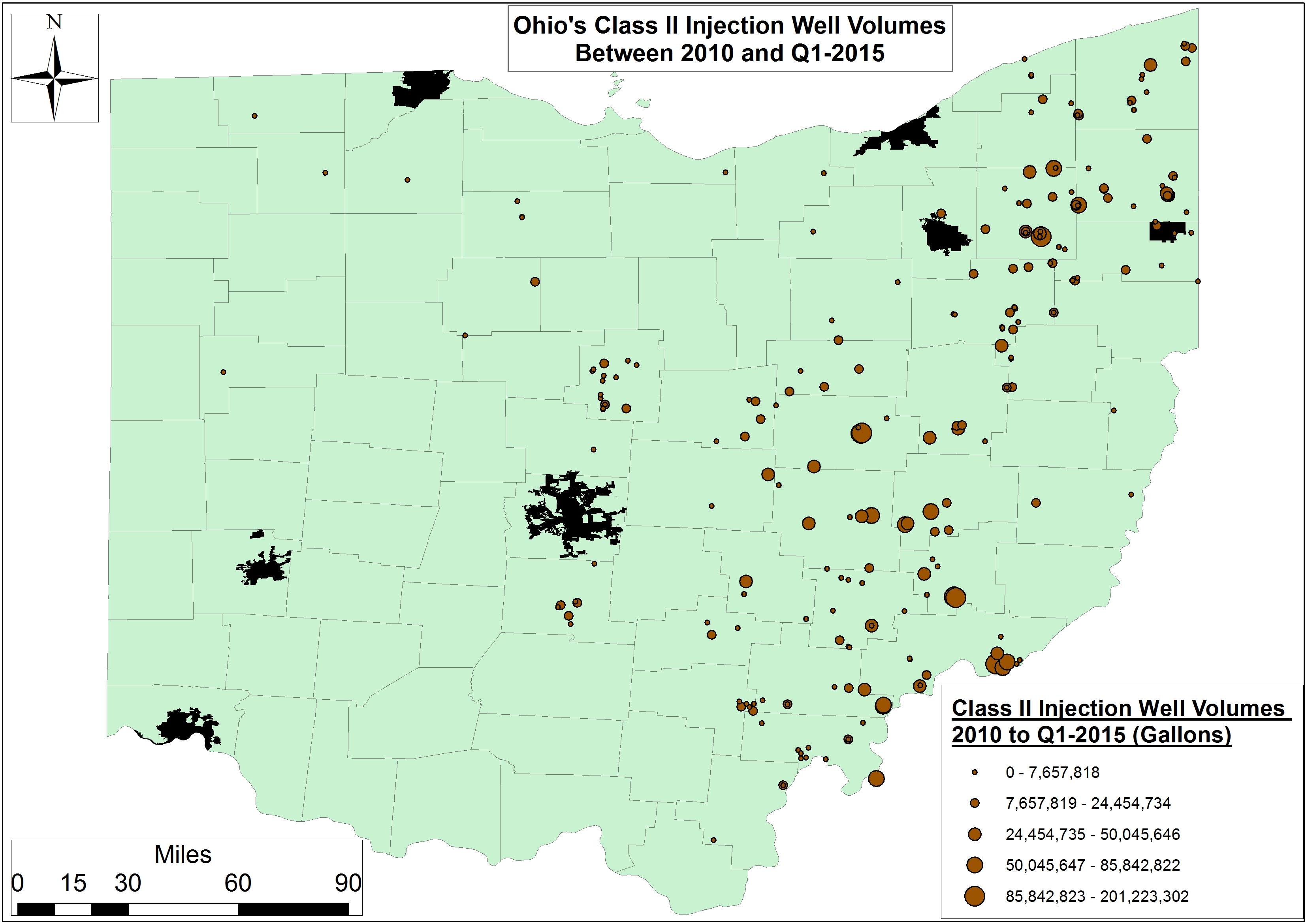
This area is also one of the top three regions of the state with respect to Class II Injection volumes; the other two high-brine production regions are Morrow and Portage counties to the west and southwest, respectively (Fig. 2).
Figure 2. Layout & Volume (2010 to Q1-2015, Gallons) of Ohio’s Active Class II Injection Wells
However, on a per-day basis we are seeing quite a few inefficient laterals across the state, including Devon Energy’s Eichelberger and Richman Farms laterals in Ashland and Medina counties. Ashland and Medina are producing 230-270 barrels (8,453-9,923 gallons) of brine per day. In Carroll County, one of Chesapeake’s Trushell laterals tops the list for brine production at 1,843 barrels (67,730 gallons) per day. One of Gulfport’s Bolton laterals in Belmont County and EdgeMarc’s Merlin 10PPH in Washington County are generating 1,100-1,200 barrels (40,425-44,100 gallons) of brine per day.
Oil & Gas Production
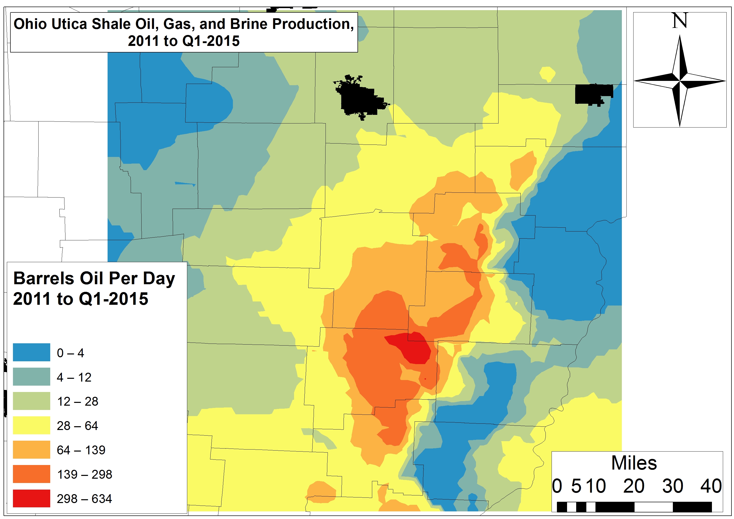
Since the last time we modeled production the oil hotspots have shrunk. They have also become more discrete and migrated southward – all of this in contrast to the model proposed by the OGS in 2012. The areas of greatest productivity (i.e., >26,000 barrels of oil) are not the central part of the state, but rather Tuscarawas, Harrison, Guernsey, and Noble counties (Fig. 1). The intersection of Harrison, Tuscarawas, and Guernsey counties is where oil productivity per-day is highest – in the range of 300-630+ barrels (Fig. 3). The areas that the OGS proposed had the highest oil potential have produced <600 barrels total or <12 barrels per day.
Figure 3. Per-Day Ohio Utica Shale Oil, Gas, and Brine Production 2011 to Q1-2015
The OGS natural gas region has proven to be another area of extremely low oil productivity.
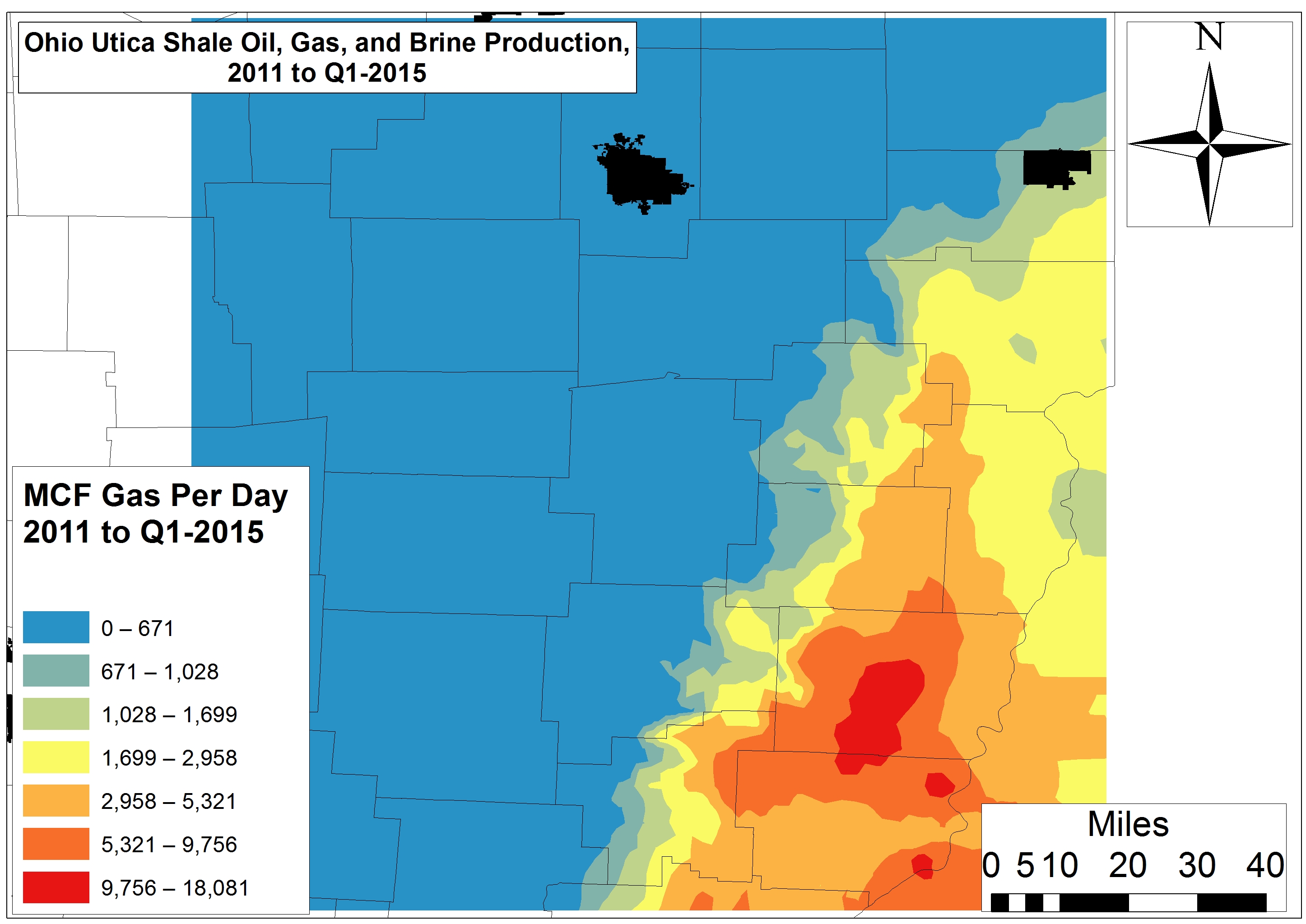
Natural gas productivity in the Utica Shale is far less extensive than the OGS projected back in 2012. High gas production is restricted to discreet areas of Belmont and Monroe counties to the tune of 947,000-4.1 million Mcf to date – or 5,300-18,100 Mcf per day. While the OGS projected natural gas and natural gas liquid potential all the way from Medina to Fairfield and Perry counties, we found a precipitous drop-off in productivity in these counties to <1,028 Mcf per day (<155,000 Mcf total from 2011 to Q1-2015) or a mere 6-11% of the Belmont-Monroe sweet spot.
Conclusion: A Shrinking Utica Shale Play
Simply put, the OGS 2012 estimates:
Have not held up,
Are behind the times and unreliable with respect to citizens looking to guestimate potential royalties,
Were far too simplistic,
Mapped high-yield sections of the “play” as continuous when in fact productive zones are small and discrete,
Did not differentiate between per day and total productivity, and
Did not address brine waste.
These issues should be addressed by the OGS and ODNR on a more transparent and frequent basis. Combine this analysis with the disappointing returns Ohio’s 17 publicly traded drilling firms are delivering and one might conclude that the structural Utica Shale bubble is about to burst. However, we know that when all else fails these same firms can just “lever up,” like their Rocky Mountain brethren, to maintain or marginally increase production and shareholder happiness. Will these Red Queens of the O&G industry stay ahead of the Big Bank and Private Equity hounds on their trail?
https://www.fractracker.org/a5ej20sjfwe/wp-content/uploads/2015/09/OH-Shrinking2-Feature.jpg400900Ted Auch, PhDhttps://www.fractracker.org/a5ej20sjfwe/wp-content/uploads/2025/09/2025-Wordmark-Logo.pngTed Auch, PhD2015-09-29 15:29:212020-03-12 17:39:58The Curious Case of the Shrinking Utica Shale Play
According to data published by the Pennsylvania Department of Environmental Protection (DEP), Pennsylvania’s unconventional oil and gas waste that was generated in the first half of 2015 found its way to treatment facilities, disposal wells, and landfills in eight different states. While the majority of the waste stayed in-state, neighboring Ohio, New York, and West Virginia all received significant quantities of both solid and liquid waste, and additional disposals were made in the non-contiguous states of Michigan, Texas, Utah, and Idaho.
Waste generated by Pennsylvania’s unconventional oil and gas wells was disposed of in a variety of ways and over a large geographic area. Click on a facility to learn more, or zoom in to access waste generated by individual wells. Click here to access the full screen map with a legend and additional controls.
Unconventional drillers in the state are now required to report production data monthly, rather than in six month increments, but waste quantities generated by the wells is still supposed to be reported biannually. However, a small number of operators have been reporting waste monthly, as well, and those figures have been included in this analysis, after spot-checking for duplication. Each record includes data on how the waste was processed and where it was shipped, so we were able to map the receiving facilities as well, and aggregate their waste totals.
Types of Waste
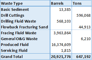
Waste generated by unconventional wells in Pennsylvania from January to June 2015 by type.
There are eight types of waste detailed in the Pennsylvania data, including:
Basic Sediment (Barrels) – Impurities that accompany the desired product
Drill Cuttings (Tons) – Broken bits of rock produced during the drilling process
Flowback Fracturing Sand (Tons) – Sand used to prop open cracks made during hydraulic fracturing that return to the surface
Fracing Fluid Waste (Barrels) – Fluid pumped into the well for hydraulic fracturing that returns to the surface. This includes chemicals that were added to the well.
Produced Fluid (Barrels) – Naturally occurring brines encountered during drilling that contain various contaminants, which are often toxic or radioactive
Servicing Fluid (Barrels) – Various other fluids used in the drilling process
Spent Lubricant (Barrels) – Oils used in engines as lubricants
General O&G Waste (Tons) – Solid waste types other than drill cuttings or fracturing sand
For the sake of simplicity, this analysis will at times aggregate the waste types into two categories, with all types reporting in tons as solid waste, while those listed in 42 gallon barrels will be considered liquid waste.
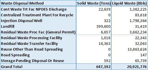
Waste Disposal
Waste disposal method for unconventional wells in PA, January to June 2015
This PA waste gets disposed of in a variety of ways. About 93 percent of all solid waste ends up in landfills. 29 of the 58 operators reporting waste during this cycle reported drill cuttings. In a separate report, the DEP has records for unconventional wells drilled by 28 different operators during the same time frame, so these results seem reasonable, since drill cuttings are generated during the drilling process, whereas other types of waste are produced throughout the life cycle of the well.
Statewide, there over 596,000 tons of drill cuttings produced during a period which saw 422 wells spudded, an average of 1,412 tons of cuttings per well. Not all operators generated the same amount of cuttings per well, however. Vantage Energy reports 3,089 tons of cuttings per well, while Hilcorp Energy manages to average just 119 tons over 23 wells drilled in the six month period. It is worth noting that some wells that were spudded just prior to the reporting period likely still generated drill cuttings during the six months in question, and some wells spudded during the cycle will continue to produce cuttings into the next one.
In terms of liquid waste, nearly two thirds of the amount reported is reused for purposes other than road spreading. This is, unfortunately, a dead end in terms of being able to follow the waste stream in the data, as there are no facilities associated with the 13.8 million barrels of waste that falls into this category. 225,000 barrels are specified as being reused for hydraulic fracturing, while the remainder is simply destined for, “Reuse without processing at a permitted facility.”
The amount used for road spreading, 147 barrels, is relatively small, and all of this waste is reported as going to private roads in Greene County. The total amount of liquid waste produced in the six month period is almost 879 million gallons, or enough to fill 1,331 Olympic-sized swimming pools.
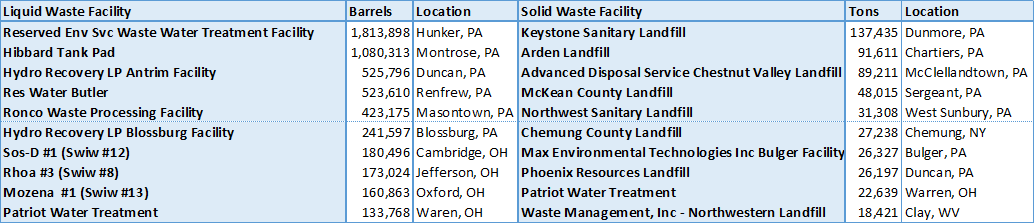
PA Waste Receiving Facilities
Altogether, we know where roughly 7 million of the nearly 21 million barrels of reported liquid waste wound up, as well as 640,000 of the 647,000 tons of solid waste. The top ten destinations for each waste type are as follows:
Top 10 reported recipients of unconventional O&G waste produced in PA during the first half of 2015.
Six of the top destinations for liquid waste were located in-state, while seven of the top ten facilities for solid waste stayed in Pennsylvania. The only facility to appear on both lists is Patriot Water Treatment in Warren, Ohio.
https://www.fractracker.org/a5ej20sjfwe/wp-content/uploads/2014/10/Waste-Data-Feature.png400900Matt Kelso, BAhttps://www.fractracker.org/a5ej20sjfwe/wp-content/uploads/2025/09/2025-Wordmark-Logo.pngMatt Kelso, BA2015-09-18 11:02:512020-03-12 13:49:50Pennsylvania’s Drilling Waste Distributed to Eight States
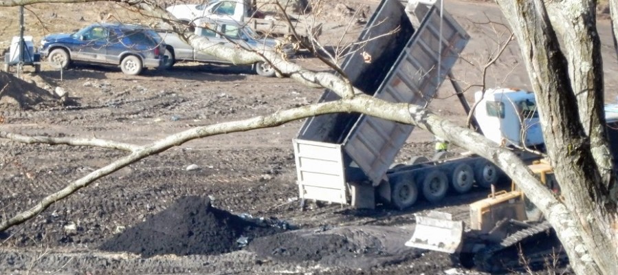
FracTracker Alliance worked with Public Herald this spring to update and map oil and gas complaints filed by citizens to the Pennsylvania Department of Environmental Protection (PA DEP) as of March 2015. The result is the largest release of oil and gas records on water contamination due to fracking in PA. Additionally, Public Herald’s investigation revealed evidence of Pennsylvania state officials keeping water contamination related to fracking “off the books.”
The mission of Public Herald, an investigative news non-profit formed in 2011, is two-fold: truth + creativity. Their work uses investigative journalism and art to empower readers and hold accountable those who put the public at risk. For this project, Public Herald aims to improve the public’s access to oil and gas information in PA by way of file reviews and data digitization. Public Herald maintains an open source website called #fileroom, where people can access a variety of digital information originally housed on paper within the PA DEP. This information is collected and synthesized with the help of donors, journalists and researchers in a collective effort with the community. To date, these generous volunteers have already donated more than 2,000 hours of their time collecting records.
The site includes complaints, permits, waste, legal cases, and gas migration investigations (GMI) conducted by the PA DEP. Additionally, there is a guide on how to conduct file reviews and how to access information through the “Right-to-Know” law at the PA DEP. They have broken down complaints and permits by county; wastes and GMI categories by cases, all of which include test results from inspections; and correspondence and weekly reports.
Some partners and contributors to the file team include Joshua Pribanic as the co-founder and Editor-in Chief, Melissa Troutman as co-founder and Executive Director, John Nicholson, who collects and researches for several databases, Nadia Steinzor as a contributor through Earthworks, and many more. Members of FracTracker working on this project include Matt Kelso, Samantha Rubright, and Kirk Jalbert.
#fileroom’s update expands the number of complaint data records collected to 18 counties – and counting!
Over the past few years, oil train traffic across the continent has increased rapidly with more than 500,000 rail cars moving oil in 2014 alone, according to the Association of American Railroads. The recent Lac-Mégantic, Quebec disaster and subsequent accidents illustrate the severity of this issue. There is a pressing need to determine true hazards facing our communities and to develop solutions to prevent further disasters. Across the United States and Canada, the issue of oil trains has quickly risen onto the agenda of community leaders, safety experts, researchers, and concerned citizens. There is much to discover and share about protecting people and vulnerable places from the various risks these trains pose. Oil Train Response 2015 provides two invaluable forums on this most pressing problem and provides information and insights for every audience.
November 13, 2015
Community Risks & Solutions Conference Presented by The Heinz Endowments
November 14 & 15, 2015
Activist Training Weekend Presented by ForestEthics
The one-day conference presented by The Heinz Endowments invites all interest groups to hear from experts about the scale and scope of this challenge, as well as updates on the current regulatory and legal frameworks; consider case studies about the actions/measures taken by various communities in response; and, participate in discussion sessions to explore solutions to better safeguard communities. Elected officials, regulators, and emergency response professionals from Pennsylvania and beyond are especially encouraged to attend to take advantage of this important learning and networking opportunity.
Training – November 14-15th
Saturday, Nov. 14th: Training 7:30 AM – 5:00 PM. Reception 6:00 – 8:00 PM
Sunday, Nov. 15th: Training 7:30 AM – 2:00 PM
A two-day training presented by ForestEthics will equip grassroots and NGO leaders from across the nation with better skills to take back to their communities, and provide critical opportunities for attendees to share winning strategies with each other. In the process of sharing, the conference will help to build both the oil train movement and support the broader environmental and social justice movements. Areas of strategic focus will include: organizing, communications, spokesperson training, data management for organizers, legal strategies, and crowd-sourced train tracking. It will also provide a structured forum for advocates fighting specific oil terminal proposals in places like Philadelphia, Baltimore, and Albany to develop shared strategies and tactics and provide all participants with the skills, knowledge and contacts they will need to carry on this work once they return home.
Oil trains are a major environmental justice issue. The conference and training will speak directly to environmental justice concerns and be inclusive of communities of color, economically disadvantaged urban and rural regions, and communities already experiencing environmental inequities. To this end, need-based travel scholarships will be provided. We are committed to developing the agenda in close consultation with our allies and attendees so that it meets their needs.
While I must commend the State for looking into this important issue, much more needs to be done, and I have serious concerns about the validity of several aspects of this study. Since the report is almost 200 pages long, I will summarize its findings and my critiques below.
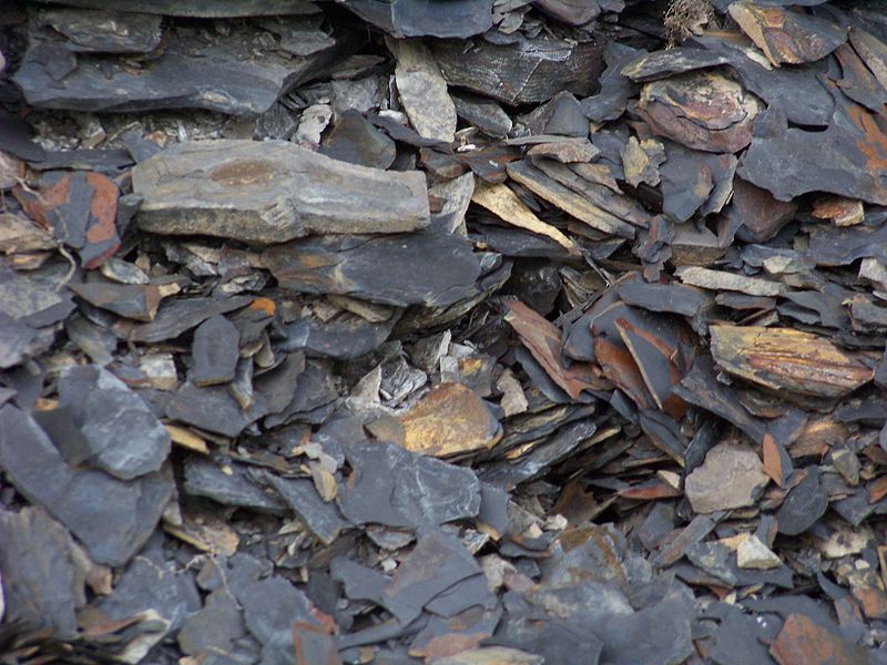
Marcellus shale cuttings are radioactive: pgs. 17, 139, 142, 154
We do not know if there is a long term problem: pg. 19
About 30 million tons of waste in next few decades: pg. 176
Landfill liners leak: pg. 20
Owning & operating their own landfill would be expensive & risky for gas companies: pgs. 186-7
Toxicity and biotic risk from drill cuttings is uncharted territory: pg. 78
Landfill leachate is toxic to plants & invertebrates: pgs. 16, 95, 97
Other landfills also have radioactive waste: pgs. 14-15
We have no idea if this will get worse: pgs. 96, 154
If all systems at landfills work as designed, leachate might not affect ground water: pg. 41
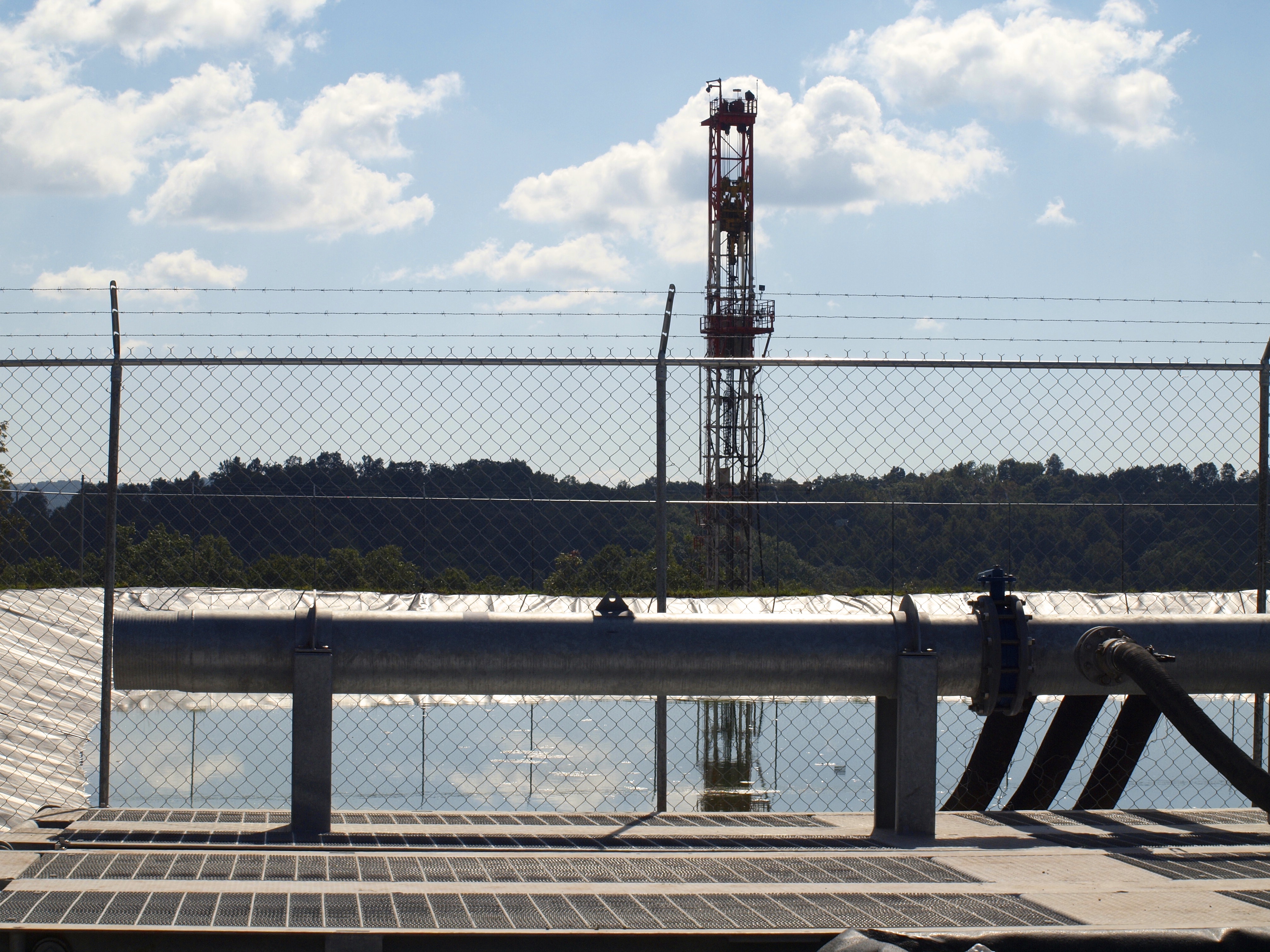
Introduction
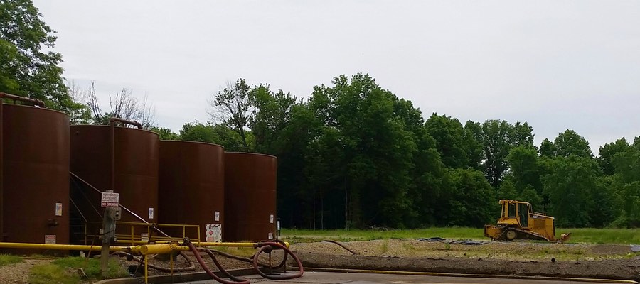
Drilling rig behind a wastewater pond in West Virginia
Any formal report comprised of 195 pages generated by a reputable school like Marshall University with additional input from Glenville State College – supported by over 2,300 pages of semi-raw data and graphs and charts and tables – requires some serious investigation prior to making comprehensive and final conclusions. However, some initial observations are needed to provide independent perspective and to help reflect on how sections of this report might be interpreted.
The overarching perspective that must be kept in mind is that the complete study was first limited by exactly what the legislature told the WV Department of Environmental Protection DEP to do. Secondly, the DEP then added other research guidelines and determined exactly what needed to be in the study and what did not belong. There were also budget and time constraints. The most constricting factor was the large body of existing data possessed by the DEP that was provided to the researchers and report writers. Because of the time restrictions, only a small amount of additional raw data could be added.
And most importantly, similar to the WVU Water Research Institute (WVU WRI) report from two years ago, it must be kept in mind that these types of studies, initiated by those elected to our well-lobbied legislature and funded and overseen by a state agency, do not occur in a political power vacuum. It was surely anticipated that the completed report might have the ability to affect the growing natural gas industry – which is supported by most in the political administration. Therefore, we must be cautious here. The presence and influence of political and economic factors need to be considered. Also, for universities to receive research contracts and government paid study requests, the focus must include keeping the customer satisfied.
My comments below on the report’s methods and findings are organized into three broad and overlapping categories:
GOOD – positive aspects, good suggestions, important observations
GENERAL – general comments
FLAW – problems, flaws, limitations
MOVING FORWARD – my suggestions & recommendations
I. Water Quality: EPA Test Protocols & Datasets
Marcellus Shale (at the surface)
GENERAL It is obvious that a very smart and well-trained set of researchers put a lot of long, detailed thought into analyzing all of the available data. There must be tens of thousands of data points. Meticulous attention was put into how to assemble all of the existing years’ worth of leachate chemical and radiological information.
GOOD There is an elaborate and detailed discussion of how to best analyze everything and how to utilize the best statistical methods and generate a uniform and integrated report. This was made difficult with non-uniform time intervals, some non-detect values, and some missing items. The researchers used a credible process, explaining how they applied the various appropriate statistical analysis methods to all the data. They provided some trends and observations and draw some conclusions.
FLAW 1 The most glaring flaw and the greatest limitation pertaining to the data sets is the nature of the very data set, which was provided to the researchers from the DEP. It is to the commendable credit of the DEP that the leachate at landfills receiving black shale drill cuttings from the Marcellus and other shale formations were, from the beginning, required to start bi-monthly testing of leachate samples at landfills that were burying drill waste products. And in general, when compared to on-site disposal as done for conventional wells, it was initially a good requirement to have the drill cuttings put into some type of landfill; that way we could keep track of where the drill cuttings are located when there are future problems.
To the best of my knowledge, until the states in the Marcellus region started allowing massive quantities of black shale waste material to be put into local landfills, we have never knowingly deposited large quantities of known radioactive industrial waste products into generic municipal waste landfills. The various waste products and drill cuttings of Marcellus black shales have been known for decades by geologists and radiochemists to be radioactive. We know better than to depose of hazardous radioactive waste in an improper way. Therefore, it is very understandable that we might not know how to best solve the problems of this particular waste product. This was and still is new territory.
FLAW 2 All of the years of leachate test samples were processed for radioactivity using what is called the clean drinking water test protocols, also referred to as the EPA 900 series. Three years ago, given the unfamiliarity of regulatory agencies with the uniqueness of this waste problem, we chose the wrong test protocol for assessing leachate samples. We speculated that the commonly used and familiar clean drinking water test procedure would work. So now we have a massive set of test results all derived from using the wrong test protocol for the radiologicals. Fortunately, all of the chemistry test results should still be reasonably useful and accurate.
At first, three years ago, this was understandable and possibly not an intentional error. Now it is widely known by hydrogeologists and radiochemists, however, that the plain EPA 900 series of test methods for determining the radioactivity of contaminated liquids do not work on liquids with high TDS — Total Dissolved Solids. Method 900.0 is designed for samples with low dissolved solid like finished drinking water supplies.
Despite this major and significant limitation, the effort by Marshall University still has some utility. For example, doing comparisons between and among the various landfills accepting drill waste might provide some interesting observations and correlations. It is clearly known now, however, that the protocols that were used for all samples from the start when testing for gross alpha, gross beta and radium-226 and radium-228 in leachate, can only result in very inaccurate, under-reported data. Therefore, it is not possible to draw any valid conclusions on several very important topics, including:
surface water quality,
potential ground water contamination,
exposure levels at landfills and public health implications,
and policy and regulations considerations.
Labs certified to test for radiological compounds and elements are very familiar with the 900 series of EPA test procedures. These protocols are intended to be used on clean drinking water. They are not intended to be used on “sludgy” waters or liquids contaminated with high dissolved solids like all the many liquid wastes from black shale operations like flowback and produced water and brines and leachate. The required lab process for sample size, preparation, and testing will guarantee that the results will be incorrect.
In no place in the final 195 page report have I seen any discussion of which EPA test protocol was used for the newer samples and why was it used. It has also not yet been seen in the 2,300+ pages of supportive statistical and analytical results, either. The fact that the wrong protocol was used three years ago is very understandable. However, this conventional EPA 900 series was still being used on the additional very recent (done in fall of 2014 and spring of 2015) samples that were included in the final report. The researchers, without any justification or discussion or explanations continued to use the wrong test protocol.
The clean drinking water procedures should have been used along with the 901.1M (gamma spec) process, for comparison. It is understandable for the new data to be consistent and comparable with the very large existing dataset that a case could be made for using the incorrect protocol and the proper one also. There should have been a detailed discussion of what and why any test method was being used, however. That discussion is usually one of the first topics investigated and explained in the Methods section. Having that type of discussion and justification seems to represent a basic science method and accepted research process – and that omission is a serious flaw.
MOVING FORWARD We all know that if we want to bake an appetizing and attractive cake we must use the correct measuring cups for the ingredients. If we want to take our child’s temperature we need an accurate thermometer. When our doctor helps us understand our blood test results, we all want to be confident the right test was used at the lab. The proper test instrument, recently calibrated and designed for the specific sample, is crucial to get useable test results from which conclusions can be drawn and policy enacted.
It seems that the best suggestion so far to test high TDS liquids similar to leachate would be to use what is referred to as Gamma-ray Spectrometry with a high purity germanium instrument with at least a 21-day hold period (30 days are better), while the sample is sealed then counted for at least 16 hours. Many of the old leachate test results indicate high uncertainties that might be attributed to short hold times and short counting times. This procedure is referred to as the 901.1 M (modified). If the sample is sealed, the sample will reach about 99% equilibrium after 30 days. Radon 222 (a gas) must not be allowed to escape.
The potential environmental impacts to water quality section of this report seems to demonstrate that if you do not want to find out something, there are always justifiable options to avoid some inconvenient facts. Given the very narrow scope as defined, some the Marshall University folks did not seem to have the option to stray into important scientific foundational assumptions and, for the most part, just had to work with the stale data sets given to them. All of which, as we have known for close to a year now, have used the wrong test protocol. Therefore we have incorrect results of limited value.
II. Marcellus is Radioactive
GOOD 1 Of course, geologists have known that the Marcellus Shale is radioactive for many decades, but also for decades there has been great reluctance by the natural gas exploration and production companies to acknowledge this fact to the public. And finally we now have a public report that clearly and unambiguously states that Marcellus shale is radioactive. Interestingly enough, it was not much more than a year ago that some on the WV House of Delegates Judiciary Committee, seemed to be echoing the industry’s intentional deception by declaring that:
…it was only dirt and rock…
So this report represents progress and provides a very valuable contribution to beginning to recognize some of the potential problems with shale wastes and their disposal challenges.
GOOD 2 Another very important advance is that finally after eight years of drilling here in Wetzel County, we now have a test sample from near the horizontal bore. The WVU WRI study researchers were never given access to any samples taken from the horizontal bore material itself, however. That was, of course, what they were supposed to have been allowed to do, but they were only given access to study material from the vertical section of the well bore. This report describes how we are getting closer to actually testing good samples of the black shale. It seems that we have gotten closer – but let’s see how close.
Page 11 describes that only three Antero wells in Doddridge County were chosen as the place to try to obtain samples from the horizontal bore. Considering that over 1,000 deviated/horizontal wells or wells with laterals have been drilled in the past few years, that number represents a very small fraction of wells drilled: less than .3%. Even if a high quality sample could have been obtained it might be a challenge to extrapolate test results to the waste being produced from the other wells in WV. These limitations are completely ignored in the report, however. Given the available documentation from the DEP, this seems to be a serious flaw that compromises the reliability of the entire report.
III. Samples From Vertical vs. Horizontal Well Bores
FLAW The actual samples tested from at least two of the three wells used in the study do not seem to be from the horizontal bore material. The sample from the third well might have come from the horizontal bore, but just barely. There is no way to know for sure. I will try to show this within the below chart using information provided by Antero to DEP Office of Oil & Gas. This information is in state records on Antero’s well plats, which become part of the well work application and also part of the final permit.
Table 1. Details about the samples taken from three Antero wells in Doddridge County, WV – and my concerns about the sampling process*
Antero well ID
API #
Sample’s drilling depth
Marcellus depth**
Horizontal bore length**
Comments / Issues
Morton 1H
47-017-06559
6,856 ft.
7,900 TVD***
10,600 ft.
~1,044 ft. short of reaching Marcellus formation
McGee 2H
47-017-06622
6,506 ft.
6,900 TVD
8,652 ft.
~394 ft. short of reaching Marcellus
Wentz1 H
47-017-06476
8,119 ft.
7,900 TVD
8,300 ft.
Just drilled into Marcellus by 219 ft.
* Original chart found on page 11 of report
** Based on information from Antero’s well plat
*** TVD = Total Vertical Depth
Antero is an active driller in Doddridge County. If any company knows where to find the Marcellus formation it is that company. Well plats are very detailed, technical documents provided to the DEP by the operator regarding the well location, watershed, and leased acres and property boundaries. We need to trust that the information on those plats is accurate and has been reviewed and approved by the permitting agency. Those plats also give the depth of the Marcellus and the length and heading of the lateral or horizontal bore. The Marshall University report gives the drilling depth when the sample was taken on the surface. Using these available well plat records from the DEP it appears that at two of the wells the sample (and its test results included in the report) came from material produced when the experienced drilling operator was not yet into the shale formation.
On the third well, Wentz 1H, the numbers seem to indicate that the sample was taken when the driller said that they were just barely within the shale layer – by 219 feet. Since the drill cuttings take some time to return to the surface from over 7,000 feet down, drilling just a few hundred feet would not at all guarantee that the returned cuttings were totally from the black shale. The processing of the drill cuttings at the shaker table and separator and centrifuge and the mixing in the tubs all cast some doubt on whether the sample, wherever it was taken from, was truly from the horizontal bore material.
On page 11 there is a clear and unambiguous statement:
Three representative sets of drill cuttings from the horizontal drilling activities within the Marcellus Shale formation were collected.
A successful attempt to get three such samples might have then allowed an appropriate waste characterization to be done as needed to accomplish the five required research topics listed in the report’s cover letter. Only an accurate chemical and radiological waste characterization would have allowed scientifically justifiable conclusions to be formulated and then allow for accurate legislation and regulations. It does not seem that West Virginia yet has the required scientific data upon which to confidently formulate laws and regulations to protect public health with regard to shale waste disposal.
Would it not seem prudent – if one wanted a good, representative sample – to make absolutely sure that the operator was, in fact, drilling in the black shale and that the cuttings returning to the surface were, in fact, from the Marcellus bore? That approach would have been eminently defensible and easily accomplished by just waiting for drilling to progress into the lateral bore far enough that the drill cuttings returning to the surface were in fact from the black shale. There might be plausible explanations for this apparent inconsistency or error. Of course, it might be speculated that the Antero-provided information on the well plats is incorrect and not intended to be accurate, or perhaps the driller is not really sure yet where the Marcellus layer starts. There may be many other possible scenarios of explanations. Time will tell.
IV. Research Observations Review
Landfill disposal of drill cuttings
GOOD There are a number of recommendations and suggestions in the study on landfills and leachate related conditions. It seems that a number of these proposals are very accurate and should be implemented. For example:
The report clearly restates that drill cuttings are known to contain radioactive compounds. Since all landfill liners will eventually leak, and since landfills already have ground water test wells for monitoring for potential ground water contamination due to leaking liners, then the well samples should be tested for radiological isotopes. Good idea. They are not required to do that now, but this recommendation should be implemented immediately (pgs. 17 and 21).
GOOD The report recommends that the Publicly Owned Treatment Works (POTW) or in the case of Wetzel County, the on-site wastewater treatment plants, should also test their effluent for radioactive isotopes. This is very important since there is no way to efficiently filter out many of the radioactive isotopes. Such contaminants will pass through traditional wastewater treatment plants.
It is also very useful that the report recommends that all the National Pollution Discharge Elimination System (NPDES) limits at the POTWs be reviewed and required to take into consideration the significantly more challenging chemical and radiological makeup of the shale waste products.
V. Economic Considerations on an Industry Supported Mono-Fill
The legislature asked that the DEP evaluate the feasibility of the natural gas industry to build, own, or operate its own landfill solely for the disposal of the known radioactive waste. This request seems to be a very reasonable approach, since for decades we have only put known radioactive waste products into dedicated landfills that are exclusively and specifically designed for the long term storage of the special waste material.
The discussion of the economic considerations is extremely complete and detailed. They are given in Appendix I and take into consideration a very thorough economic feasibility study of such a proposed endeavor. This section seems to have been compiled by a very talented professional team.
FLAW However, some of the basic assumptions are a bit askew. For example:
The initial Abstract of the financial analysis states that two new landfills would be needed because we do not want to have the well operators to drive any further than they do now. Interesting. This seems to be not too different than a homeowner while in search for privacy and quiet, builds a home far out into the country and then expects the public sewage lines to be extended miles to his new home so he would not have to incur the cost of a septic system. Homebuilders in rural settings should know they will have to incur expenses for their waste disposal needs. Should gas companies expect that communities to provide cheap waste disposal for them?
More than 15 pages later, the most important aspect is clearly stated that, “…the most salient benefit of establishing a separate landfill sited specifically to receive (radioactive) drill cuttings would be the preservation of existing disposal capacity of existing fills for future waste disposal”. Meaning for my (our) grandchildren. See page 175.
Comprehensive and sound financial details later explain that having the natural gas operators build, operate, and eventually close their own radioactive waste depository landfill would involve a lot of their capital and involve some risk to them. It is stated that their money would be better used drilling more wells. The conclusion then seems to be that, all around, it is simply cheaper and less risky for the gas industry to put all their waste products into our Municipal Waste Landfills, and later residents should incur the costs and risk to build another land fill for their household garbage when needed.
VI. Report Omissions
Within the report section dealing with the leachate test results, it is casually mentioned that not only do the landfills receiving shale waste materials have radioactive contaminated leachate, but the other tested landfills do, as well. However, rather than raising a very red flag and expressing concern over a problem that no one has looked into, the report implies we should not worry about any radioactive waste because it might be in all landfills (pg. 139).
Nowhere within the radiological discussion is there any mention of what might be called speciation of radioactive isotopes. The report does state that the test for both gross alpha and gross beta, are considered a “scanning procedure.” The speciation process is sort of a slice and dice procedure, showing exactly what isotopes are responsible for the activity that is being indicated. This process, however, does not seem to have been done on the landfill leachate test samples. The general scanning process cannot do that. Appendix H, pages 141-142, contains detailed facts on radiation dose, risk, and exposure. This might have been a good place to also discuss the proper EPA testing protocols, used or not used, and why.
A short discussion of the DEP-required landfill entrance radiation monitors is included on page 146. The installed monitors are the goalpost type. Trucks drive between them at the entrance and when they cross the scales. It seems that the report should have emphasized that that type of monitor will primarily only detect high-energy gamma radiation. However what is omitted on page 144 is that the primary form of decay for radium-226 is releasing alpha particles. The report is ambiguous in saying the decay products of radium-226 include both alpha particles and some gamma radiation, but radium-266 is not a strong gamma emitter. It is very unlikely that a normal steel enclosed roll-off box would ever trip the alarm setting with a load of drill cuttings. However those monitors are still useful since they will detect the high-energy gamma radiation from a truck carrying a lot of medical waste (pg. 17).
It is stated on page 144 that the greatest health risk due to the presence of radium-226 is the fact that its daughter product is radon-222. Radium-226 has a half-life of 1,600 years, compared to radon’s 3.8 days. This difference might seem to imply that radon is less of a concern. Given the multitude of radium-226 going into our landfills means that we will be producing radon for a very long time.
https://www.fractracker.org/a5ej20sjfwe/wp-content/uploads/2015/05/Drill-cuttings-at-landfill-3894-crop-e1432757459333.jpg400899FracTracker Alliancehttps://www.fractracker.org/a5ej20sjfwe/wp-content/uploads/2025/09/2025-Wordmark-Logo.pngFracTracker Alliance2015-08-18 09:06:432020-03-12 14:04:17Landfill Disposal of WV Oil and Gas Waste – A Report Review
Ohio waterways face headwinds in the form of hydraulic fracturing water demand and waste disposal
By Ted Auch, PhD – Great Lakes Program Coordinator, and Elliott Kurtz, GIS Intern and University of Michigan Graduate Student
In just 44 of its 88 counties, Ohio houses 1,134 wells – including those producing oil and natural gas and Class II injection wells into which the industry’s waste is disposed. Last month we wrote about Ohio’s disturbing fracking waste disposal trend and the disproportionate influence of neighboring states. (Prior to that Ariel Conn at Virginia Tech outlined the relationship between Class II Injection Wells and induced seismicity on FracTracker.) This time around, we are digging deeper into how water demand is related to Class II disposal trends.
Ohio’s Utica oil and gas wells are using 7 million gallons of freshwater – or 2.4-2.8 million more than the average well cited by the US EPA.1 Below we explore the inter-county differences of the water used in these oil and gas wells, and how demand compares to residential water demand and wastewater production.
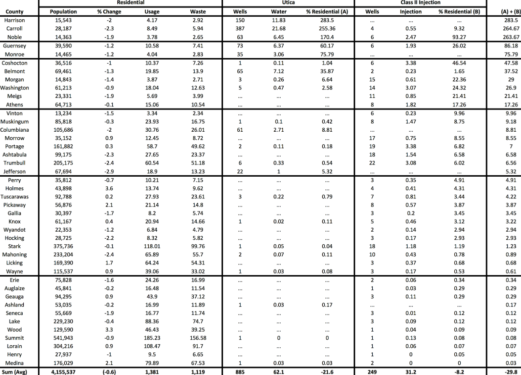
Please refer to Table 1 at the end of this article regarding the following findings.
Utica Shale Freshwater Demand
Data indicate that there may be serious threats to Ohio’s water security on the horizon due to the oil and gas industry.
The counties of Guernsey and Monroe are next up with water demand and waste water generation at rates of 14.6 and 10.3 million gallons per year. However, the 11.4 million gallons of freshwater demand and fracking waste produced by these two counties 114 Utica and Class II wells still accounts for roughly 81% of residential water demand.
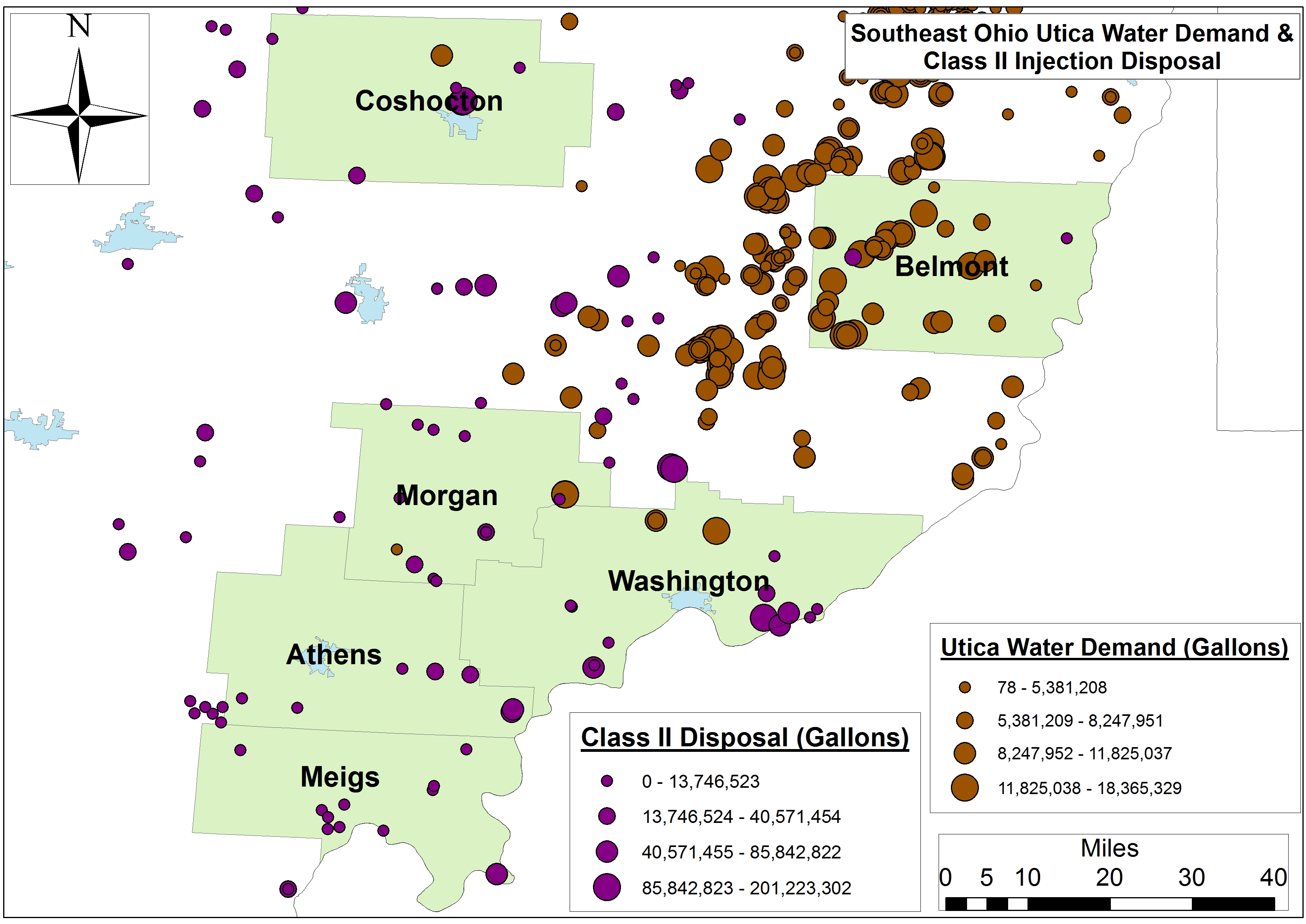
The wells within the six-county region including Meigs, Washington, Athens, and Belmont along the Ohio River use 73 million gallons of water and generate 51 million gallons of wastewater per year, while the hydraulic fracturing industry’s water-use footprint ranges between 48 and 17% of residential demand in Coshocton and Athens, respectively. Class II Injection well disposal accounts for a lion’s share of this footprint in all but Belmont County, with injection well activities equaling 77 to 100% of the industry’s water footprint (see Figure 1 for county locations and water stress).
Figure 1. Primary Southeast Ohio counties experiencing Utica Shale and Class II water stress
The next eight-county cohort is spread across the state from the border of Pennsylvania and the Ohio River to interior Appalachia and Central Ohio. Residential water demand there equals 428 million gallons, while the eight county’s 92 Utica and 90 Class II wells have accounted for 15 million gallons of water demand and disposal. Again the injection well component of the industry accounts for 5.8% of the their 7.7% footprint relative to residential demand. The range is nearly 10% in Vinton and 5.3% in Jefferson County.
The next cohort includes twelve counties that essentially surround Ohio’s Utica Shale region from Stark and Mahoning in the Northeast to Pickaway, Hocking, and Gallia along the southwestern perimeter of “the play.” These counties’ residents consume 405 million gallons of water and generate 329 million gallons of wastewater annually. Meanwhile the industry’s 69 Class II wells account for 53 million gallons – a 2.8% water footprint.
Finally, the 11 counties with the smallest Utica/Class II footprint are not suprisingly located along Lake Erie, as well as the Michigan and Indiana border, with water demand and wastewater production equalling nearly 117 billion gallons per year. Meanwhile the region’s 3 Utica and 18 Class II wells have utilized 59 million gallons. These figures equate to a water footprint of roughly 00.15%, more aligned with the 1% of total annual water use and consumption for the hydraulic fracturing industry cited by the US EPA this past June.
Future Concerns and Projections
Industry will see their share of the region’s hydrology increase in the coming months and years given that injection well volumes and Utica Shale demand is increasing by 1.04 million gallons and 405-410 million gallons per quarter per well, respectively. The number of people living in these 42 counties is declining by 0.6% per year, however, 1.4% in the 10 counties that have seen the highest percentage of their water resources allocated to Utica and Class II operations. Additionally, hydraulic fracturing permitting is increasing by 14% each year.2
Table 1. Residential, Utica Shale, and Class II Injection well water footprint across forty-two Ohio Counties (Note: All volumes are in millions of gallons)
2. Auch, W E, McClaugherty, C, Gallemore, C, Berghoff, D, Genshock, E, Kurtz, E, & Jurjus, R. (2015). Ramification of current and future production, resource utilization, and land-use change in the Ohio Utica Shale Basin. Paper presented at the National Environmental Monitoring Conference, Chicago, IL.
https://www.fractracker.org/a5ej20sjfwe/wp-content/uploads/2015/08/InjectionWells-Feature.jpg400900Ted Auch, PhDhttps://www.fractracker.org/a5ej20sjfwe/wp-content/uploads/2025/09/2025-Wordmark-Logo.pngTed Auch, PhD2015-08-11 10:42:442020-03-12 14:04:43Threats to Ohio’s Water Security
In February 2014, the FracTracker Alliance produced our first version of a national well data file and map, showing over 1.1 million active oil and gas wells in the United States. We have now updated that data, with the total of wells up to 1,666,715 active wells accounted for.
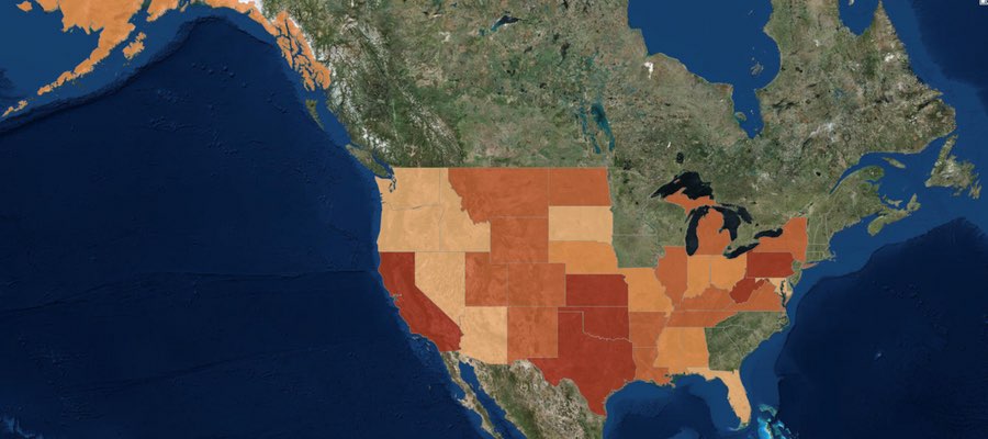
Density by state of active oil and gas wells in the United States. Click here to access the legend, details, and full map controls. Zoom in to see summaries by county, and zoom in further to see individual well data. Texas contains state and county totals only, and North Carolina is not included in this map.
While 1.7 million wells is a substantial increase over last year’s total of 1.1 million, it is mostly attributable to differences in how we counted wells this time around, and should not be interpreted as a huge increase in activity over the past 15 months or so. Last year, we attempted to capture those wells that seemed to be producing oil and gas, or about ready to produce. This year, we took a more inclusive definition. Primarily, the additional half-million wells can be accounted for by including wells listed as dry holes, and the inclusion of more types of injection wells. Basically anything with an API number that was not described as permanently plugged was included this time around.
Data for North Carolina are not included, because they did not respond to three email inquiries about their oil and gas data. However, in last year’s national map aggregation, we were told that there were only two active wells in the state. Similarly, we do not have individual well data for Texas, and we use a published list of well counts by county in its place. Last year, we assumed that because there was a charge for the dataset, we would be unable to republish well data. In discussions with the Railroad Commission, we have learned that the data can in fact be republished. However, technical difficulties with their datasets persist, and data that we have purchased lacked location values, despite metadata suggesting that it would be included. So in short, we still don’t have Texas well data, even though it is technically available.
Wells by Type and Status
Each state is responsible for what their oil and gas data looks like, so a simple analysis of something as ostensibly straightforward as what type of well has been drilled can be surprisingly complicated when looking across state lines. Additionally, some states combine the well type and well status into a single data field, making comparisons even more opaque.
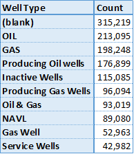
Top 10 of 371 published well types for wells in the United States.
Among all of the oil producing states, there are 371 different published well types. This data is “raw,” meaning that no effort has been made to combine similar entries, so “gas, oil” is counted separately from “GAS OIL,” and “Bad Data” has not been combined with “N/A,” either. Conforming data from different sources is an exercise that gets out of hand rather quickly, and utility over using the original published data is questionable, as well. We share this information, primarily to demonstrate the messy state of the data. Many states combine their well type and well status data into a single column, while others keep them separate. Unfortunately, the most frequent well type was blank, either because states did not publish well types, or they did not publish them for all of their wells.
There are no national standards for publishing oil and gas data – a serious barrier to data transparency and the most important takeaway from this exercise…
Wells by Location
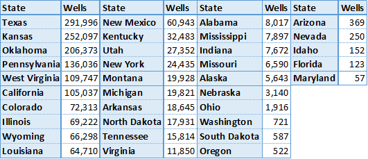
Active oil and gas wells in 2015 by state. Except for Texas, all data were aggregated published well coordinates.
There are oil and gas wells in 35 of the 50 states (70%) in the United States, and 1,673 out of 3,144 (53%) of all county and county equivalent areas. The number of wells per state ranges from 57 in Maryland to 291,996 in Texas. There are 135 counties with a single well, while the highest count is in Kern County, California, host to 77,497 active wells.
With the exception of Texas, where the data are based on published lists of well county by county, the state and county well counts were determined by the location of the well coordinates. Because of this, any errors in the original well’s location data could lead to mistakes in the state and county summary files. Any wells that are offshore are not included, either. Altogether, there are about 6,000 wells (0.4%) are missing from the state and county files.
Wells by Operator
There are a staggering number of oil and gas operators in the United States. In a recent project with the National Resources Defense Council, we looked at violations across the few states that publish such data, and only for the 68 operators that were identified previously as having the largest lease acreage nationwide. Even for this task, we had to follow a spreadsheet of which companies were subsidiaries of others, and sometimes the inclusion of an entity like “Williams” on the list came down to a judgement call as to whether we had the correct company or not.
No such effort was undertaken for this analysis. So in Pennsylvania, wells drilled by the operator Exco Resources PA, Inc. are not included with those drilled by Exco Resources PA, Llc., even though they are presumably the same entity. It just isn’t feasible to systematically go through thousands of operators to determine which operators are owned by whom, so we left the data as is. Results, therefore, should be taken with a brine truck’s worth of salt.
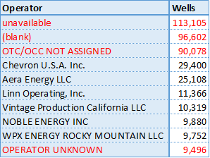
Top 10 wells by operator in the US, excluding Texas. Unknown operators are highlighted in red.
Texas does publish wells by operator, but as with so much of their data, it’s just not worth the effort that it takes to process it. First, they process it into thirteen different files, then publish it in PDF format, requiring special software to convert the data to spreadsheet format. Suffice to say, there are thousands of operators of active oil and gas wells in the Lone Star State.
Not counting Texas, there are 39,693 different operators listed in the United States. However, many of those listed are some version of “we don’t know whose well this is.” Sorting the operators by the number of wells that they are listed as having, we see four of the top ten operators are in fact unknown, including the top three positions.
Summary
The state of oil and gas data in the United States is clearly in shambles. As long as there are no national standards for data transparency, we can expect this trend to continue. The data that we looked for in this file is what we consider to be bare bones: well name, well type, well status, slant (directional, vertical, or horizontal), operator, and location. In none of these categories can we say that we have a satisfactory sense of what is going on nationally.
Click on the above button to download the three sets of data we used to make the dynamic map (once you are zoomed in to a state level). The full dataset was broken into three parts due to the large file sizes.
https://www.fractracker.org/a5ej20sjfwe/wp-content/uploads/2015/08/2015Update-Feature.jpg400900Matt Kelso, BAhttps://www.fractracker.org/a5ej20sjfwe/wp-content/uploads/2025/09/2025-Wordmark-Logo.pngMatt Kelso, BA2015-08-03 14:19:532020-07-21 10:30:051.7 Million Wells in the U.S. – A 2015 Update
By Ted Auch, Great Lakes Program Coordinator, and Elliott Kurtz, GIS Intern
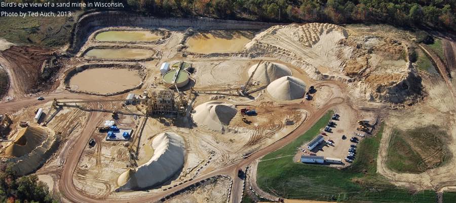
The Great Lakes may see a major increase in the number of sand mines developed in the name of fracking. What impacts has the area already seen, and does future development mean for the region’s ecosystem and land use?
Wisconsin’s 125+ silica sand mines and processing facilities are spread out across 15,739 square miles of the state’s West Central region, adjacent to the Minnesota border in the Northern Mississippi Valley. These mines have dramatically altered the landscape while generating proppant for the shale gas industry; approximately 2.5 million tons of sand are extracted per mine. The length of the average shale gas lateral well grows by > 50 feet per quarter, so we expect silica sand usage will grow from 5,500 tons to > 8,000 tons per lateral. To meet this increase in demand, additional mines are being proposed near the Great Lakes.
Migration of the sand industry from the Southwest to the Great Lakes in search of this silica sand has had a large impact on regional ecosystem productivity and watershed resilience[1]. The land in the Great Lakes region is more productive, from a soil and biomass perspective; much of the Southwest sandstone geology is dominated by scrublands that have accrue plant biomass at much slower rates, while the Great Lakes host productive forests and agricultural land. Great Lakes ecosystems produce 1.92 times more soil organic matter and 1.46 times more perennial biomass than Southwestern ecosystems.
Effects on the Great Lakes
Quantifying what the landscape looks like now will serve as a baseline for understanding how the silica sand industry will have altered the overall landscape, much like Appalachia is doing today in the aftermath of strip-mining and Mountaintop Removal Mining[2]. West Central Wisconsin (WCW) has a chance to learn from the admittedly short-cited and myopic mistakes of their brethren across the coalfields of Appalachia.
Herein we aim to present numbers speaking to the diversity and distribution of WCW’s “working landscape” across eight types of land-cover. We will then present numbers speaking to how the silica mining industry has altered the region to date and what these numbers mean for reclamation. The folks at UC Berkeley’s Department of Environmental Science, Policy , and Management describe “Working Landscapes” as follows:
a broad term that expresses the goal of fostering landscapes where production of market goods and ecosystem services is mutually reinforcing. It means working with people as partners to create landscapes and ecosystems that benefit humanity and the planet… A goal is finding management and policy synergies—practices and policies that enhance production of multiple ecosystem services as well as goods for the market…Collaborative management processes can help discover synergies and create better decisions and policy. Incentives can help private landowners support management that benefits society.
Methods
We used the 1993 WISCLAND satellite imagery to determine how WCW’s landscape is partitioned and then we applied these data to an updated inventory of silica sand mine boundaries to determine what existed within their boundaries prior to mining. The point locations of Wisconsin’s current inventory of silica sand mines was determined using the “Geocode Address” function in ArcMap 10.2 using the Composite_US Address Locator. Addresses were drawn from mine inventory information originally maintained by the West Central WI Regional Planning Commission (WCWRPC) and now managed by the WI Department of Natural Resources’ Mines, pits and quarries division. Meanwhile current mine extent boundary polygons were determined using one of three satellite data-sets:
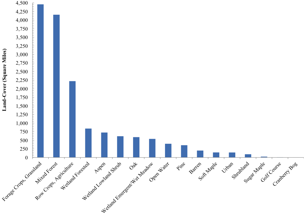
Fig 1. Square mileage of various land cover types replaced by silica sand mining in WCW
Thirty-nine percent of the WCW landscape is currently allocated to forests, 43% to agriculture broadly speaking, and 13% is occupied by various types of wetlands. Open waters occupy 2.6% of the landscape with tertiary uses including barren lands (1.3%), golf courses (0.03%), high and low-density urban areas (0.9%), and miscellaneous shrublands (0.6%) (See Figure 1).
Effects by Land Cover Type
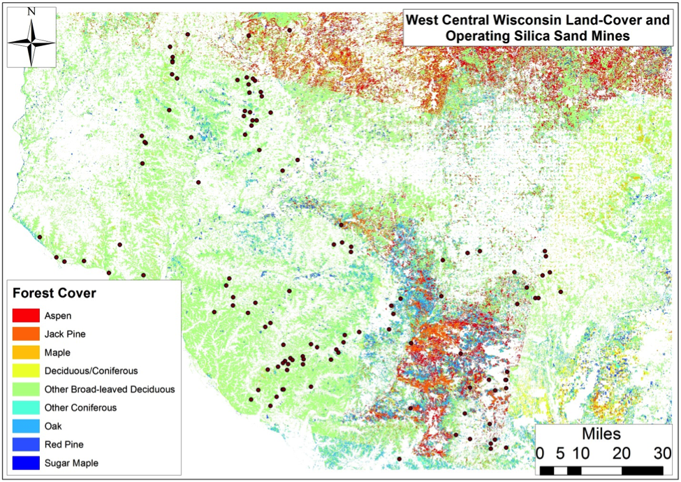
Fig 2. Forest Cover in WCW
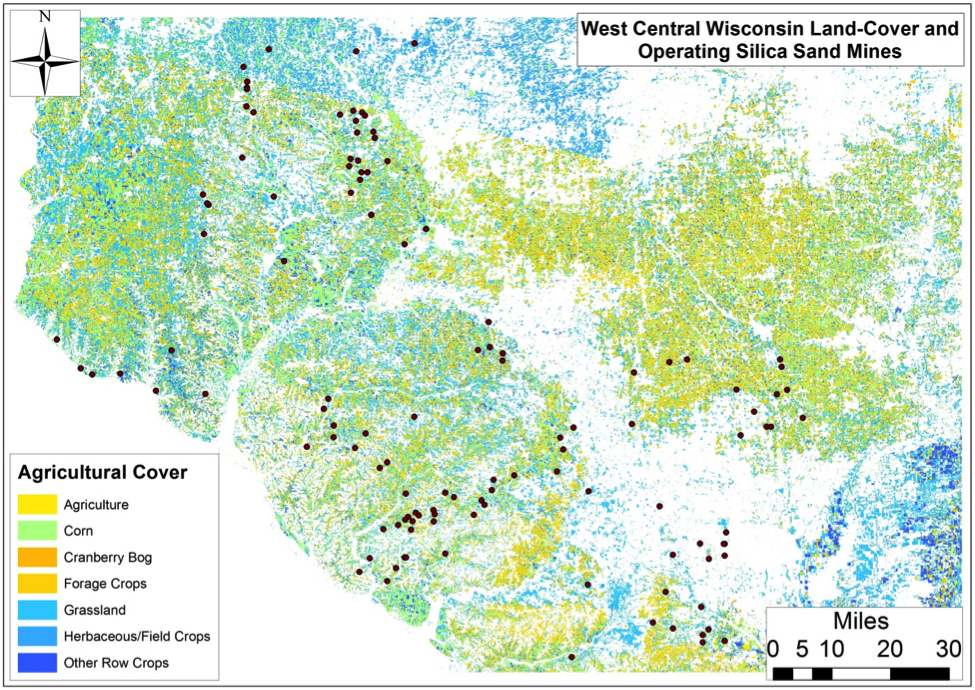
Fig 3. Agricultural Cover
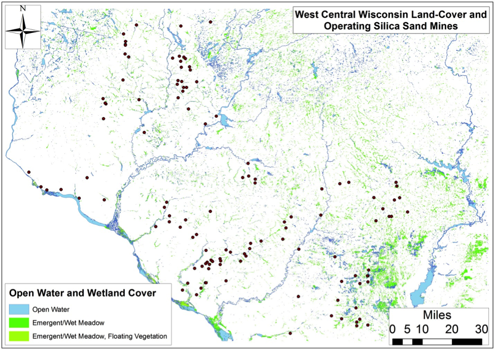
Fig 4. Open Water & Wetland Cover
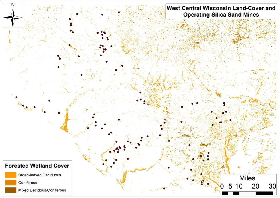
Fig 5. Forested Wetland Cover
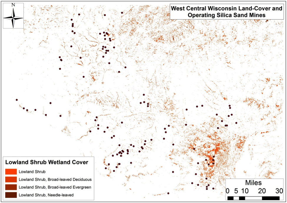
Fig 6. Lowland Shrub Wetlands
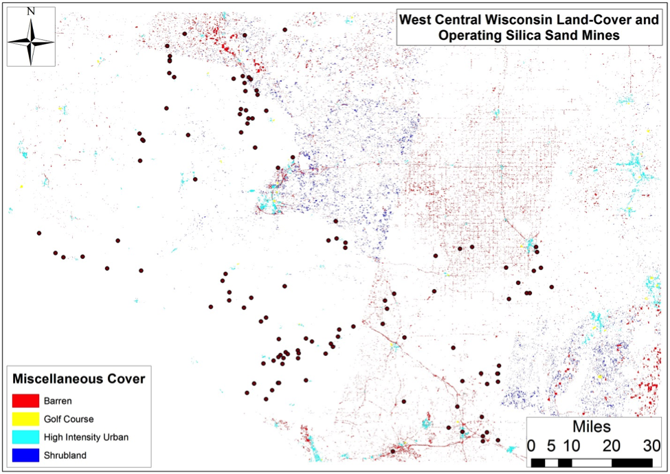
Fig 7. Miscellaneous Cover
Figure 2. The wood in these forests has a current stumpage value of $253-936 million and by way of photosynthesis accumulates 63 to 131 million tons of CO2 and has accumulated 4.8-9.8 billion tons of CO2 if we assumed that on average forests in this region are 65-85 years old. Putting a finer point on WCW forest cover and associated quantifiables is difficult because most of these tracts (2.7 million acres) fall within a catchall category called “Mixed Forest”. Pine (2.3% of the region), Aspen (4.7%), and Oak (3.8%) most of the remaining 1.2 million forested acres with much less sugar (Acer saccharum) and soft (Acer rubrum) maple acreage than we expected scattered in a horseshoe fashion across the Northeastern portion of the study area.
Figure 3. Seven different agricultural land-uses occupy 4.3 million WCW acres with forage crops and grasslands constituting 29% of the region followed by 1.4 million acres of row crops and miscellaneous agricultural activities. Additionally, 2% of WI’s 19,700 cranberry bog acres are within the study area generating $4.02 million worth of cranberries per year. The larger agricultural categories generate $3.2 billion worth of commodities.
Figure 4. Nearly 16% of WCW is characterized by open waters or various types of wetlands with a total area of 2,396 square miles clustered primarily in two Northeast and one Southeast segment. Open waters occupy 398 square miles with forested wetlands – possibly vernal pool-type systems – amounting to 5.4% of the region or 841 square miles. Lowland shrub and emergent/wet meadows occupy 540 and 618 square miles, respectively.
Figure 5. Of the nine types of wetlands present in this region the forested broad-leaved deciduous and emergent/wet meadow variety constitute the largest fraction of the region at 1,107 square miles (7.1% of region). Some percentage of the former would likely be defined by Wisconsin DNR as vernal pools, which do the following according to their Ephemeral Pond program. The WI DNR doesn’t include silica sand mining in its list of 14 threats to vernal pools or potential conservation actions, however.
These ponds are depressions with impeded drainage (usually in forest landscapes), that hold water for a period of time following snowmelt and spring rains but typically dry out by mid-summer…They flourish with productivity during their brief existence and provide critical breeding habitat for certain invertebrates, as well as for many amphibians such as wood frogs and salamanders. They also provide feeding, resting and breeding habitat for songbirds and a source of food for many mammals. Ephemeral ponds contribute in many ways to the biodiversity of a woodlot, forest stand and the larger landscape…they all broadly fit into a community context by the following attributes: their placement in woodlands, isolation, small size, hydrology, length of time they hold water, and composition of the biological community (lacking fish as permanent predators).
Figure 6. Broad-leaved evergreen lowland shrub wetlands constitute ≈2.1% of the region or 319 square miles with most occurring around the Legacy Boggs silica mines and several cranberry operations turned silica mines in Jackson County. Meanwhile broad-leaved deciduous and needle-leaved lowland shrub wetlands are largely outside the current extent of silica sand mining in the region occupying 1.9% of the region with 293 square miles spread out within the northeastern 1/5th of the study area.
Figure 7. Finally, miscellaneous land-covers include 200 square miles of barren land, 145 square miles of low/high intensity urban areas including the cities of Eau Claire (Pop. 67,545) and Stevens Point (Pop. 26,670) as well as towns like Marshfield, Wisconsin Rapids, Merrill, and Rib Mountain-Weston. WCW also hosts 3,204 acres (0.03% of region) worth of golf courses which amounts to roughly 21 courses assuming the average course is 157 acres. Shrublands broadly defined occur throughout 0.6% of the region scattered throughout the southeast corner and north-central sixth of the region, with the both amalgamations poised to experience significant replacement or alteration as they are adjacent to two large silica mine groupings.
Producing Mine Land-Use/Land-Cover Change
To date we have established the current extent of land-use/land-cover change associated with 25 producing silica mines occupying 12 square miles of WCW. These mines have displaced 3 square miles of forests and 7 square miles of agricultural land-cover. These forested tracts accumulated 31,446-64,610 tons of CO2 per year or 2.4-4.9 million tons over the average lifespan of a typical Wisconsin forest. These values equate to the emissions of 144,401-295,956 Wisconsinites or 2.5-5.1% of the state’s population. The annual wood that was once generated on these parcels would have had a market value of $126,097-197,084 per year. Meanwhile the above agricultural lands would be generating roughly $1.5-3.3 million in commodities if they had not been displaced.
However, putting aside measurable market valuations it turns out the most concerning result of this analysis is that these mines have displaces 871 acres of wetlands which equals 11% of all mined lands. This alteration includes 158 acres of formerly forested wetlands, 352 acres of lowland shrub wetlands, and 361 acres of emergent/wet meadows. As we mentioned previously, the chance that these wetlands will be reconstituted to support their original plant and animal assemblages is doubtful.
We know that the St. Peter Sandstone formation is the primary target of the silica sand industry with respect to providing proppant for the shale gas industry. We also know that this formation extend across seven states and approximately 8,884 square miles, with all 91 square miles overlain by wetlands in Wisconsin. To this end carbon-rich grasslands soils or Mollisols, which we discussed earlier, sit atop 36% of the St. Peter Sandstone and given that these soils are alread endangered from past agricultural practices as well as current O&G exploration this is just another example of how soils stand to be dramatically altered by the full extent of the North American Hydrocarbon Industrial Complex. The following IFs would undoubtedly have a dramatic effect on the ability of the ecosystems overlying the St. Peter Sandstone to capture and store CO2 to the extent that they are today not to mention dramatically alter the landscape’s ability to capture, store, and purify precipitation inputs.
IF silica sand mining continues at the rate it is on currently
IF reclamation continues to result in “very poor stand of grass with some woody plants of very poor quality and little value on the whole for wildlife. Some areas may be reclaimed as crop land, however it is our opinion that substantial inputs such as commercial fertilizer as well as irrigation will be required in most if not all cases in order to produce an average crop.”
IF the highly productive temperate forests described above are not reassembled on similar acreage to their extent prior to mining and reclamation is largely to the very poor stands of grass mentione above
For example: Great Lakes forests like the ones sitting atop the St. Peter Sandstone capture 20.9 tons of CO2 per acre per year Vs their likely grass/scrublands replacement which capture 10.6-12.8 tons of CO2 per acre per year… You do the math!
“None two sites are capable of supporting the growing of food. They grow trees and some cover grass, but that is all. General scientific research says that the reclaimed soils lose up to 75% of their agricultural productivity.”
Quote from a concerned citizen:
I often wonder what it was like before the boom, before fortunes were built on castles of sand and resultant moonscapes stretched as far as the eye could see. In the past few years alone, the nickname the “Silica Sand Capital of the World” has become a curse rather than a blessing for the citizens of LaSalle County, Illinois. Here, the frac sand industry continues to proliferate and threaten thewellbeing of our people and rural ecosystem.
The US Forest Service defined Watershed Resilience as “Over time, all watersheds experience a variety of disturbance events such as fires and floods [and mining]. Resilient watersheds have the ability to recover promptly from such events and even be renewed by them. Much as treating forests can make them more resilient to wildfire, watershed restoration projects can improve watershed resilience to both natural and human disturbances.”
https://www.fractracker.org/a5ej20sjfwe/wp-content/uploads/2015/07/SandMine-WI-Feature.jpg400900Ted Auch, PhDhttps://www.fractracker.org/a5ej20sjfwe/wp-content/uploads/2025/09/2025-Wordmark-Logo.pngTed Auch, PhD2015-07-16 14:24:562020-03-12 14:05:24West Central Wisconsin’s Landscape and What Silica Sand Mining Has Done to It