Life and Times of Loyalsock
By Brook Lenker, Executive Director, and Samantha Malone, Manager of Science and Communications
It’s so quiet you can hear moss squish underfoot and the tapping of a woodpecker a quarter-mile distant. These are the sounds of a lesser-known Pennsylvania Wilds, the lush woodlands and rock-studded beauty of the Loyalsock State Forest. Picture a pristine landscape of ferny grottos, expansive bogs, and blueberries ripe for the picking. The squeaky-clean air seems hyper-enriched, a photosynthetic side-effect of stands thick with maple, birch, hemlock, and pine. Currents of endless streams race impatiently. Rattlesnakes shy but leery, lie and rest.
Across Lycoming and Sullivan counties, the shale gas industry is leaving its industrial footprint, from the iconic Pine Creek Valley through Tiagdaghton State Forest to the Loyalsock and environs. Yet while Williamsport booms from the infusion of gas, many of the hidden, ecologically-rich spaces of the Loyalsock – from Rock Run to Devil’s Elbow – still whisper.
According to the Pennsylvania Department of Conservation and Natural Resources (DCNR), of the 2.2 million acres in the state forest system, 675,000 acres are available for gas development. This includes 385,400 acres under Commonwealth-issued leases and 290,000 acres of where the agency doesn’t own the oil and gas rights. The latter scenario applies to 25,621 acres of the Loyalsock’s 114,494 acres where “severed” rights are owned by Anadarko Petroleum Corporation and International Development Corporation.
 Circa July 2012, there is ample evidence of the changes on the horizon. The oranges and yellows of seismic testing equipment (photo left) adorn the sleepy forest roads and the electric pink of ribbon markers decorates the trees and ground. The few leased cabins look lost and lonely, but soon they could have the steady companionship of hundreds of trucks rumbling past their doors carrying water, sand, and some not-so-benign chemicals and waste fluids. The narrow, dirt roads – bound to require widening and repair – are probably inadequate for such intensive use and potentially treacherous for heavy rigs, occasionally known to roll down steep embankments and spill their secrets. Heavy traffic and structurally-degraded roads can cause significant sediment pollution as suggested by the studies of the Penn State Center for Dirt and Gravel Roads. Sediment is the enemy of native brook trout, our handsome state fish, who adamantly require cool, clear water to survive. Currently, there’s an abundance of such good water within Loyalsock.
But traffic and roadway impacts are but one piece of the shale gas puzzle. Could well casings fail and methane bubble into surface waters (recent accidents in Bradford County and Tioga County are suspected of causing just such problems)? How much will air quality be degraded by diesel emissions from trucks, pumps, generators, drill rigs, and other equipment? How will floodlights and flaring affect star-packed skies or the incessant drone of compressor stations antagonize solitude? While off the beaten path, the forest sees its share of visitors, and recreational trails are a signature of the region. The 27-mile Old Logger’s Path (photo below) is a backpacker’s dream crisscrossing a world of palpable wonders and subterranean severed rights.

Hiking, a popular recreation, and the forest’s quality scenery are big components of tourism, consistently one of Pennsylvania’s leading industries. According to the Pennsylvania Tourism Office, visitor spending across the Commonwealth totaled $34.2 billion in 2010. Comparatively, Penn State research (p.31) indicated that, “…the Marcellus gas industry increased Pennsylvania’s value added by $11.2 billon” for 2010. In the northeastern Pennsylvania, drilling is slowing due in part to the low price of natural gas. The ramifications for the Loyalsock are uncertain but the lasting attraction of idyllic open spaces is unequivocal.
Nevertheless, Anadarko and its partner seek the gas near the Old Loggers Path and vulnerable populations of forest interior birds. Such species require large unbroken tracts of contiguous forest. A recent study in Environmental Management authored by P.J. Drohan, Margaret Brittingham, and others reports that 26% of well pads in the Susquehanna basin are located in core forests (many on DCNR lands). The study quotes a DCNR paper: “further (shale gas) development on state forests is likely to alter the ecological integrity and wild character of state forests.” The authors believe other research supports that assertion.
The Loyalsock is a microcosm of the state forest-shale gas paradigm. As of a March 2012 DCNR presentation, 814 Marcellus well locations had been approved by the Bureau of Forestry on state forest land and 447 Marcellus wells had been drilled in the state forests including more than 80 well pads. The agency estimates a total of 3810 new Marcellus wells by 2018. With an average well pad size of about five acres, many miles of new and widened roads, even more miles of pipelines, plus intermittent water impoundments and compressor stations, it’s easy to wonder what our state forests will soon look like. And what about the legacy of silviculture cultivated by Pinchot, Rothrock, and other conservation pioneers? The Pennsylvania state forest system is certified by the Rainforest Alliance under Forest Stewardship Council standards ensuring that the products coming from these forests are managed in an environmentally-responsible manner. At what threshold of shale gas activity will this certification – which adds significant value to finished wood products – be jeopardized?
Since it is likely that Anadarko and its partner will pursue their claims, the fate of the severed parts of the Loyalsock may be shaped by the existence or lack-thereof of a surface use agreement between Anadarko and DCNR. Where DCNR has leased and controls oil and gas rights, a surface use agreement is entered into that steers the development activity in a more sustainable manner and away from especially sensitive forest features. In the case of severed rights, there is uncertainty about the applicability of surface use agreements. However, with little else to ameliorate the collateral damage of gas development in undeveloped surroundings, prudence would suggest it’s a tool worth using.
The stakes are high. DCNR’s own list of “challenges” posed by shale gas for state forest lands include: surface disturbance, forest fragmentation, habitat loss and species impacts, invasive plants, loss of wild character, recreation conflicts, water use and disposal. With the mission of the Bureau of Forestry to “ensure the long-term health, viability and productivity of the Commonwealth’s forests and to conserve native wild plants,” they have their work cut out for them, especially as more drilling tracts are developed.
In the months to come, the industry will be watched, technologies will change, activists will speak, parties will talk; meanwhile, the big, old rattlers, wise but weary, grow restless.