Data and Analysis Archives - Page 18 of 22

Data driven discussions about gas extraction and related topics.

2010 Fines for Marcellus Shale Violations

May 16, 2011/by Matt Kelso, BA

In yesterday’s Post-Gazette, Don Hopey discussed an analysis by PennFuture which saw a notable decline in fines in the first quarter of 2011, as compared to the same period last year. The implication is that the DEP is not backing up violations with fines under Governor Corbett’s administration to the same degree that it did under former Governor Rendell. In the former administration, PennFuture calculated an enforcement action was handed out for every 1.7 violations, and now the rate is one per every 8.7 violations.

I think this is a worthwhile trend to keep an eye on, with the caveat that it is still early in Governor Corbett’s tenure, and that violation data varies widely from month to month.

It is also possible that the DEP under the Corbett administration will still issue fines for significant events. In fairness, I came across this article of fines issued over eight months after an incident by the DEP under Rendell. I think we need more time to see if the new administration’s patterns of reduced fines per violation hold.

That said, Marcellus Shale fines and enforcements under the Rendell administration is hardly a sensible target for comparison. The fines issued in 2010 were at once paltry and erratic.

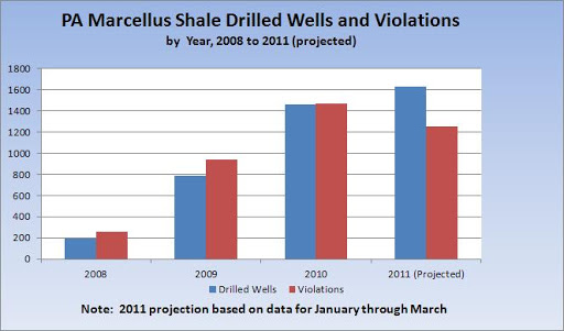
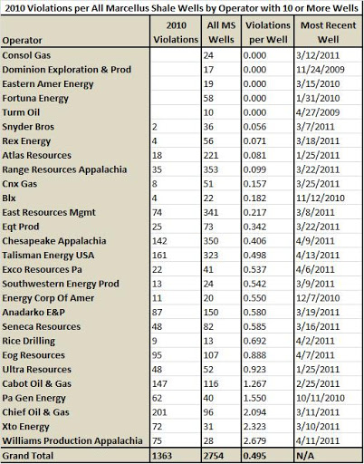
Industry sources indicate that Marcellus Shale wells cost between $5 million to $6.4 million to drill. Last year in Pennsylvania, there were 1,454 Marcellus Wells drilled in the Commonwealth, meaning that the total cost of operations for the year for the industry is somewhere in the mind-boggling range of $7.2 billion to $9.3 billion. How much of that cost was fines issued by the DEP? $775,650.22. Even using the conservative figure of $5 million per well, DEP fines only account for 0.01 percent of operating costs–hardly any impediment at all. In essence, with the change in administration the DEP went from collecting fines in Monopoly money to asking drilling operators to sit down for a while and think about what they’ve done.

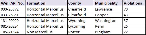
Over 45 percent of the fines issued for the Marcellus Shale in 2010 went to EOG Resources, the operator for a major blowout in Clearfield County. That was far from the only major incident in 2010, but the DEP was clearly mad about the incident, posting an entire section about the incident on their website. The $353,400 fined to EOG for this incident went to cover the DEP’s cost of response and investigation.

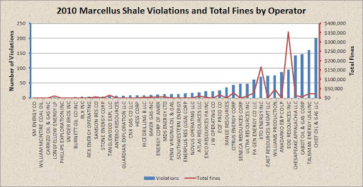
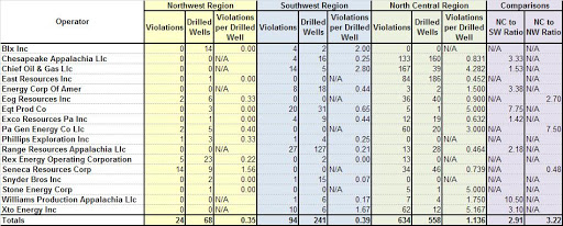
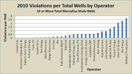
The two operators with the highest fines issued for Marcellus Shale operation in 2010 are toward the top of companies with the largest number of violations per year. That said, those companies at the very top were fined a significantly lower amount.

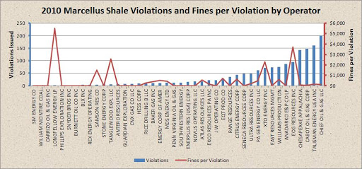
When we look at fines per violation, in addition to the same two operators that stood out in the last graph, we see several companies with relatively few violations having a significant number of fines per violation.

From an outside perspective, it is difficult to determine what sorts of factors go into whether or not a fine is issued, and if so, for how much. If the goal is simply to recoup costs of the DEP response and investigation, one wonders why there isn’t a fine more often, since every violation issued costs the DEP some resources to evaluate, process, and issue. And if fines are to act as a deterrent, they should include punitive damages, not just actual costs.

Keep in mind that the $7.2 billion to $9.3 billion range is just for Marcellus Shale wells, which last year represented about half of all oil and gas wells drilled in Pennsylvania. The industry is huge. One way we could have the oil and gas industry benefit all Pennsylvanians is by paying for the expenses of their DEP oversight, through permit fees and fines. That taxpayer savings could then be applied to other programs to help address the overall budget issue. Such an arrangement would be a huge boon to Pennsylvania, and while they might complain, the industry would barely notice if their cost per well went up by a few thousand dollars. Such an arrangement would also allow for the DEP to keep up with a rapidly expanding industry in a time of fiscal austerity that is sweeping the Commonwealth, and the nation as a whole.

Other sources, such as the Marcellus Drilling News report higher fine totals, but that includes a broader time frame. See Sean Hamill’s Post-Gazette article.

Issuance of PA Marcellus Shale Violations Over Time and by DEP Region

May 4, 2011/by Matt Kelso, BA

Changes Over TimeEvery time I think about the number of violations issued by the Pennsylvania Department of Environmental Protection (DEP) Bureau of Oil and Gas Management, I am struck on the one hand by the sheer magnitude of them–last year, the DEP issued 2,704 violations(1), a number that everyone would like to see go way down in the years ahead. On the other hand, at least that means the DEP is paying attention. It is with this spirit that I delved into the numbers, hoping to find patterns either in time or space.

The DEP has only occasionally issued more Marcellus Shale violations per month than for other combined oil and gas formations.

The monthly issuance of violations is surprisingly erratic in a industry that is accelerating drilling activity steadily, especially for the Marcellus Shale. Once we look at the data on an annual basis, though, a clearer picture begins to emerge.

Based on a projection from the first quarter of 2011, this year will be the first year with more new Marcellus Shale wells drilled than DEP violations issued.

The number of drilled Marcellus Shale wells in Pennsylvania has been growing rapidly since the first well was drilled in 2006. Violations have been on the rise as well, but if the projections for 2010 hold true, there will actually be fewer violations this year than last year, despite the fact that there will be more Marcellus wells drilled. Again, due to the erratic nature of violations issued per month, such a projection should be taken with a grain of salt. On the other hand, it does fit with the long term trend of Marcellus Shale violations issued per wells drilled for the same calendar year.

The number of Marcellus Shale violations per well has been decreasing over time, as has the budget of the Pennsylvania Department of Environmental Protection.

This graph is an attempt to look into the issue of whether the trend of decreasing violations per well might be due to DEP budget(2) issues rather than an overall increase in compliance by the industry. While this graph does not answer the question, it does lend the notion credibility.

Variance by DEP Region

Although there are six DEP regions, the Bureau of Oil and Gas is active out of three of them: the Northwest Regional Office (NWRO), the Southwest Regional Office (SWRO), and the North Central Regional Office (NCRO). All oil and gas activity in other portions of the state are included with the NCRO, giving them by far the largest territory to cover.

Violations per Well

Marcellus Shale violations per well by issuing DEP region. Click on the map for a larger, dynamic view.

The NCRO issued more than three times as many violations per Marcellus Shale well in 2010 than either of the other two regional offices. This is despite having the largest territory, and, as it turns out, the heaviest Marcellus Shale workload (3).

Violations per Inspection

DEP workload by region.

Number of Marcellus Shale inspections and wells drilled in 2010 by DEP Region.

Each DEP Oil and Gas Region had at least twice as many inspections as new drilled wells for the Marcellus Shale in 2010.

Marcellus Shale violations per inspection by issuing DEP region. Click the image for a larger, dynamic view.

The North Central Regional Office issued over eight times as many violations per inspection for Marcellus Shale wells as either of the other two DEP offices in 2010, despite the heaviest Marcellus Shale inspection workload.

Enforcement

The NCRO issued more than twice as many enforcement actions per inspection for Marcellus Shale wells than either the SWRO or NWRO in 2010.

As a quick review of the numbers for the Marcellus Shale from 2010, the NCRO compares to the other regions by issuing more than:

Three times as many violations per well
Eight times as many violations per inspection
Two times as many enforcement actions per inspection

The DEP briefly entertained the notion of centralizing violations and enforcement actions of Marcellus Shale wells. One wonders whether the end result would have been to reduce the vigilance of the NCRO, or whether the SWRO and NWRO would be instructed to catch up with their sibling. Indeed, either course of action could occur, even without Secretary Krancer’s direct approval of such actions.

Operators Active in Multiple Regions

Although the violation and enforcement numbers of the NCRO above are already convincing, there is another variability that could potentially skew the data: drilling operators. Some of the better operators in terms of violations per well such as Consol and Range Resources are active primarily in the SWRO’s jurisdiciton. Could it be that the NCRO just has more bad apples than the other two regions?

To answer this, I narrowed the list of Marcellus Shale operators from wells drilled in 2010 to those active in more than one region, the results of which are below.

There were 17 drilling operators that drilled Marcellus Shale wells in more than one DEP oil and gas region in 2010.

Even when we limit the field to the eleven operators active in the NCRO and one of the other districts, we once again see that the North Central Regional Office issued about three times as many violations per well as did the others.

Drilling operators with at least one 2010 Marcellus Shale well in the NCRO as well as either the SWRO or NWRO. Seneca Resources is the only instance where there were fewer violations issued in the NCRO than elsewhere.

It seems difficult to imagine that the geology in the NCRO jurisdiction is really that much more challenging to work with than the rest of the state. Short of that, I cannot speculate on a reason for the consistently stark contrast in violation and enforcement patterns other than to suggest that the North Central Regional Office is run with a culture of vigilance that is unmatched by their counterparts in the Southwest and Northwest.

The goal should be for the industry to achieve a greater level of compliance with Pennsylvania’s environmental laws, not to see a greater number of violations. At the same time, every person deserves to know that he or she is being aggressively protected from an industry that can be very dangerous and polluting. Undoubtedly, there is a lot that goes into the inspection process beyond the issuance of violations and enforcement actions, and the numbers can only go so far in providing a description of events on the ground. Nonetheless, those numbers are striking and consistent in showing a North Central Regional Office that takes a no-nonsense approach to its efforts of regulating the Marcellus Shale industry, at least as compared to either the Southwest Regional Office and Northwest Regional Office.

The numbers from this summary page do not match exactly with the DEP violations page data for 2010.
I would have rather compared violations to the Bureau of Oil and Gas budget, but it is not separated in that fashion within the budget reports.
The NCRO does have the smallest overall workload, but this blog is focused on the Marcellus Shale.

PA Marcellus Shale Violations by Operator and County

April 21, 2011/by Matt Kelso, BA

Archived

This post has been archived.

Earlier this month, I examined 2010 oil and gas violation data for Pennsylvania on a summary level. Now I’m going to focus just on Marcellus Shale wells, and from the perspective of trying to determine the extent that drilling operators and location have on the likelihood of increased violations for any given well.

There are a number of ways in which this could be done. Although I am interested to see if the number of wells drilled in an area or by a drilling operator has a noticeable effect on violations, I have limited both investigations to 10 or more Marcellus Shale wells, both to avoid the erratic results of small sample sizes, and because the large number of results tends to make for crowded data displays.

Violations are only for 2010, both because it is current, and with 1,544 records, it is sufficiently large to make some generalizations about. As for wells, I decided to go for all drilled Marcellus Shale wells rather than just the 2010 wells, because wells that were spudded between 2006 and 2009 might well be included on the violations list. Also, the overall number of wells is a handy way to gauge the relative weight of a given operator or county on the industry as a whole.

2010 Marcellus Shale (MS) violations per total MS well, for counties with 10 or more MS wells.

2010 MS violations per total MS well, for operators with 10 or more MS wells.

There are, of course, a number of issues once we start looking at the data in detail. One of the biggest challenges is that many of these wells change hands, or else the companies that drill them change hands or are no longer active in the Marcellus Shale drilling industry in Pennsylvania. For example, in a previous analysis, I noted that Turm Oil had a large number of violations per well, and now they had none at all. I checked to see when their most recent well was drilled, and found my answer:

List of operators with 10 or more MS wells, with 2010 violations, frequencies per well, and the date of the most recent well drilled

Turm Oil hasn’t drilled a Marcellus well in almost two years. Looking at the chart above, Turm and Dominion don’t really belong in this analysis, and Eastern American and Fortuna may not for 2011. These four operators account for everyone with 10 or more total Marcellus Shale wells and no violations in 2010 except for Consol—kudos to Consol!

Does the number of wells impact violations?

Clearly, there is a tremendous range of violations per well, both in regards to who the operator is, as well as where the well is located. My hypothesis going into this analysis was that the more wells an operator drilled or the more wells drilled in a county, the fewer violations per well there would be.

I had several reasons for suspecting this to be the case. First of all, think of what must be done for a drilling operation without violations being issued. The site must be carefully placed, in accordance with all applicable regulations. The site must be prepared, taking into account all ground disturbing regulations. Then you have to drill through thousands of feet of rock, making sure that there is a structurally sound casing and cementing job to prevent gas migrations. Then there is the horizontal drilling, and the hydraulic fracturing. All along the way, not a drop of fracing fluid, diesel fuel, brine, or really anything else can touch the ground or enter Pennsylvania’s waters in any way. And when the drilling is done, the site must be restored in a timely fashion. And those are just a few of the regulations that the drilling operators agree to when they undertake drilling operations in Pennsylvania.

Let’s face it—that’s a lot to achieve. In order to consistently come in and out of a site with a clean record has got to take some practice. I’ve heard from industry sources that Marcellus Shale wells cost about $5 million to drill, so to do it right without cutting corners clearly takes significant resources as well.

In addition to all of that, a county level map of Marcellus Shale violations per well shows that the counties which produce the most Marcellus Shale gas wells are not the ones with the highest number of violations per well.

Map showing Marcellus Shale violations per county. Counties outlined in red have 100 or more Marcellus Shale wells. Click the gray compass rose and double carat (^) to hide those menus.

So is there then any correlation between the number of wells drilled and the violations issued? Let’s take a look (1).

The equations for the trendlines were calculated by Excel, and I selected the ones with the highest R-squared values. I was surprised that the best fit for operators was a convex polynomial. In the graph above, there is indeed a cluster of operators with between 300 and 400 wells, and with about 0.5 violations per well or less, but on the other end of the spectrum, the violations per well are spread far apart. There are so many operators big and small with around 0.5 violations per well or less that it seems some other factors must be at play for all of the operators that exceed that value by a significant margin. Perhaps not everyone will achieve zero violations like Consol did in 2010, but it doesn’t seem reasonable that Williams Production Appalachia should have more than twice the amount of violations as Range Resources Appalachia, despite having only 8 percent of the number of wells as the gas extraction giant.

The correlation was a bit stronger for the counties than for the operators. I’m not entirely sure what factors are at play here, other than perhaps having a crew that is well familiar with the geology of the region and all the specific challenges associated with that. Again though, that doesn’t seem to explain why Wyoming County would have 3.44 violations for every Marcellus Shale well, while those in Washington county can only expect a violation for less than one well out of eight drilled.

[photo removed]

Again, I’m sure that the way this analysis was set up had an effect on some of these numbers, and Wyoming is certainly a smaller sample size than Washington. I also don’t want to infer that there aren’t problems when large operators drill in well established portions of the Marcellus Shale. What’s more, while over 1,500 Marcellus Shale violations in a year is a huge number, it likely doesn’t account for all of the actual incidents, just the ones that the DEP can demonstrate, apparently beyond a shadow of a doubt (2). And even in the best scenario, there are significant impacts upon the land and neighboring residents near the well site.

I am suggesting, however, that there are companies that need to do better in their efforts to comply with laws designed to protect Pennsylvanians from pollution and other deleterious effects of oil and gas drilling. Excuses that environmental regulations are too strict don’t hold water, as their competitors are closer to compliance, sometimes dramatically so.

In order for Excel to be able to calculate all of the various regression lines, counties and operators with zero violations per well had to be excluded from this analysis.
I have personally talked to numerous residents who feel that their well water was spoiled by gas operations on neighboring lands. A common theme in their complaints is that the DEP places the burden of proof on residents that their wells were not spoiled before drilling operations began–an almost impossible situation for the residents to predict and be proactive about.

How Long Between MS Permit Issuance and Drilling in PA?

April 14, 2011/by Matt Kelso, BA

2011 Marcellus Shale drilled wells (green circles) and permits issued (red stars). For a larger, dynamic view, please click the image.

All Marcellus Shale permits issued (red circles) and drilled wells (green circles). Please zoom in for a closer look in the denser portions of the map.

Sometimes it seems like the oil and gas industry is in an awfully big hurry. They are in a hurry to get the mineral leases, presumably because if they don’t, some other operator will. They are in a hurry to get their drilling permits from the Department of Environmental Protection (DEP)–already this year, the DEP has issued 979 permits from the Marcellus Shale formation alone. And sometimes they are in a hurry to get the drill in the ground. Sometimes, however, they are not.

This does not mean that I think the 444 Marcellus Shale wells that have been spudded (time when the drill first hits the ground) so far this year is a small number. After all, today is just the 104th day of the year, which means that on average, almost 4.3 Marcellus Shale wells are started every single day. That’s a lot of industrial activity, and yet it reflects well under half of the 9.5 Marcellus Shale permits that DEP secretary Michael Krancer signs off on every day.

The longer term trends are similar: Of the 6,092 Marcellus Shale wells with active permits(1), 2,574 have been drilled. That represents about 42 percent, meaning that the 45 percent clip for 2011 is actually running a bit ahead of schedule. All of this brings a couple questions to mind:

Why does the oil and gas industry get more than twice as many permits as they are able to drill?
What’s the lag time for drilling once the permit is in hand?

I’m still scratching my head over the first one. I have been told that the siting and permitting processes are so involved and expensive that once the permit is in hand, the industry will drill the site, but the numbers don’t seem to reflect that as being fully true. Certainly, the 107 oil and gas drilling rigs available in Pennsylvania right now is a limiting factor in how many wells are drilled, but that doesn’t explain why the permitting process is years ahead of the drilling queue.

As for how long it takes to drill once a permit has been issued, there are means of answering that question. First, I matched the permits data to the spuds data using the wells’ unique API numbers, finding 2,804 matches for 2,574 distinct wells (2)(3). The second step was to subtract the number of days between the spud date and the permit date to determine the lag time for those permits which have been drilled, and where API numbers did match up. Let’s take a look at the results:

Number of days between permit issuance and spud (initial drilling) date.

Some of the 39 wells marked as “reworked” may not have originally been Marcellus Shale wells, so they were not included in the chart above. In addition, there were two negative values, for which it would appear that well was drilled before the permit was issued. I am assuming those are attributable to clerical error, and those wells were not included in the chart above (4).

Number of days from permit issuance to spud date for Marcellus Shale wells. Please click the “i” and then a map feature for more information. Please click the gray compass rose and double carat (^) to hide those menus.

Overall, the value ranges from -86 to 2,274 days, with an average turnaround time of just over 100 days. If we omit the outliers discussed above, the values range from 1 to 566 days, with an average of just under 99 days.

After looking at these results, I am surprised by the vast range, and beyond the number of available rigs, I can only speculate as to what factors go into determining this. It also seems remarkable that there are wells that can get the equipment in place, the site prepared, and the drill in the ground the very next day after the permit was issued. And yet, for all of that celerity, sometimes it takes well over a year to start churning dirt.

This data comes from the DEP’s Operators With Active Wells Inventory section of their Reports page. What I called “active permits” are actually “active wells” according to the DEP. These include all wells for which the permit has been issued but have not yet been plugged. This would include wells that hav not been drilled, thus my distinction.
Both datasets had some duplication of well numbers. All records that were exact duplicates were removed, meaning that the remainder had at least slight variances in one or more columns.
I should mention that the number of matches to the permits list means that there are 93 mismatches between the two datasets. In theory, all of the drilled wells should be on the permit report, but for now, let’s take the 97% match rate and move forward.
All values are included in the posted dataset, and therefore the DataTool map.

Proposed Tire Fire Plant in Greenwood Twp., Crawford County, PA

April 12, 2011/by FracTracker Alliance

In the fall of 2010 Crawford Renewable Energy, LLC (CRE) announced plans to build a “tire-fired” power plant in Greenwood Township of Crawford County. The facility is designed to produce 100 MW of energy by burning used, recycled tires in two circulating fluidized bed (CFB) boiler systems. The design of the facility includes several pollutant emission control technologies. These types of equipment remove a portion of the pollutants from the exhaust. As nice as it is to think of tires simply “disappearing” rather than being land-filled, when any hydrocarbon fuel source is burned, such as a tire or coal, a multitude of toxic and carcinogenic compounds are released. And most of these pollutants cannot be captured using control technologies, so they are emitted into the air.

The facility is planned on an 80 acre industrial park land parcel. The control equipment includes a CFB scrubber, a fabric filter baghouse, and a regenerative catalytic reactor. The flue gasses will then be emitted through a 325 foot tall stack. A CFB scrubber uses limestone to decrease sulfur emissions. The regenerative catalytic reactor is used to reduce NO_X. The fabric filter baghouse is a series of screens and filters that remove the majority of the mass of particulate matter. The majority of the mass of particulate emissions are removed by capturing the coarse fraction of particles, which are particles with larger diameters and mass, but do not pose a significant health threat. Baghouses and other particulate control devices (PCDs) are not as efficient at capturing the fine and ultrafine fraction of particulate emissions, which have smaller diameters. The fine and ultrafine modes of particulates are the most hazardous, and are directly related to asthma exacerbation, chronic obstructive pulmonary disorder (COPD) and other forms of respiratory disease.

The emissions and deposition pattern from this facility were modeled by the Center for Healthy Environments and Communities to assess the impact on local air quality. Several pollutant species were modeled, including sulfur dioxide (SO₂), oxides of nitrogen (NO_x), and both the course and the fine fractions of particulate matter, PM₁₀ and PM_2.5 respectively. Concentrations of these pollutants at ground level in ambient air were modeled using the CalPUFF non-steady state dispersion model. These will not be the only pollutants transported, rather these are efficient to model. Plumes of some of the other contaminants will most likely have similar patterns.

The mean, or average, levels of predicted ambient air concentrations are presented first for each pollutant (Figures 1, 3, 5, and 7). These maps show the average concentrations of the pollutant that are predicted to occur while the facility is operating. The concentrations are averaged over a one year period. Next, peak day concentrations of pollutants are presented (Figures 2, 4, 6, and 8). These concentrations are the highest predicted concentrations for a single day that would occur when the facility is operating normally, over the one year modeled cycle. The concentrations shown in all of the maps are only attributable to the proposed facility, and do not include any other sources of pollution or background concentrations of pollutants. These values essentially show the increases in ambient air pollutants that will occur when the proposed facility is operating.

For this 80 acre industrial park, a square “fence-line” with 570 meter sides could surround the park. Typically, exposures are expected to be very limited within the fence-line because the area is inaccessible to the public. Concern is focused on the exposures that may occur beyond the limit of the fence-line. If the smokestack is assumed to be located at the center of the park, it would be at a distance approximately 235 meters from the fence-line. Using the scales on the maps, it is evident that the even the highest concentration gradients shown in the maps would occur beyond the fence-line. When the facility is operating, it is reasonable for the surrounding communities to expect exposures to even the highest concentration gradients shown in the maps.

Figure 1. Mean values of modeled SO₂ ambient air concentrations at ground level, attributable to emissions from the proposed CRE plant.

Figure 2. Peak day values of modeled SO₂ ambient air concentrations at ground level, attributable to emissions from the proposed CRE plant.

Figure 3. Mean values of modeled NO_X ambient air concentrations at ground level, attributable to emissions from the proposed CRE plant.

Figure 4. Peak day values of modeled NO_X ambient air concentrations at ground level, attributable to emissions from the proposed CRE plant.

Figure 5. Mean values of modeled PM₁₀ ambient air concentrations at ground level, attributable to emissions from the proposed CRE plant.

Figure 6. Peak day values of modeled PM₁₀ ambient air concentrations at ground level, attributable to emissions from the proposed CRE plant.

Figure 7. Mean values of modeled PM_2.5 ambient air concentrations at ground level, attributable to emissions from the proposed CRE plant.

Figure 8. Peak day values of modeled PM_2.5 ambient air concentrations at ground level, attributable to emissions from the proposed CRE plant.

A Look at Horizontal Well Production in Virginia

April 11, 2011/by Matt Kelso, BA

Horizontal gas wells in Virginia in 2008 to 2009. Note that they are all clustered in the extreme western portion of the Commonwealth.

According to the Virginia Department of Mines, Minerals, and Energy’s (DMME) Division of Gas and Oil, there are 30 horizontal gas wells that produced gas between January 2008 and December 2009 (1). While this is not a large number of horizontal wells, the dataset is interesting, since Virginia publishes monthly production data online.

Of the 30 wells, only nine were in production for at least 12 of the 24 months that I looked at. This is, admittedly, a small sample size, but is as good an entry point as any into the discussion of how gas production changes over time.

Chart 1: Production in Thousands of Cubic Feet (Mcf) of Horizontal Gas Wells in Virginia, with at least 12 months of production between 2008 to 2009.

Many of the wells in this analysis have a spike in production within the first few months of production, followed by a gradual decline.

Chart 2: Maximum, Minimum, and Mean Production of Horizontal Gas Wells in Virginia, with at least 12 months of production between 2008 to 2009.

For wells with at least 12 months of production, the mean production value tends to be closer to the minimum value than the maximum. This is particularly true for those wells which show a significant spike in production, such as VH-520008.

Chart 3: Ratio of Most Recent Monthly Production to Peak Monthly Production of Horizontal Gas Wells in Virginia, with at least 12 months of production between 2008 to 2009.

Ratio of December 2009 production to each well’s maximum monthly production for all horizontal gas wells. Please click the gray compass rose and double carat (^) to hide those menus. Click the “i” tool then any map feature for more information.

For these nine horizontal gas wells in Virginia, the average production of the most recent month (December 2009) is slightly less than 30 percent of the peak monthly production. This figure is skewed on the one side by a well with a tremendous production spike (VH-530008, 6.93%) and on the other by a well with low but relatively steady production (VH-536927, 42.75%). When all wells are considered (as with the map) the range of values is much greater.

Each of these wells had been in production between 12 and 24 months as of December 2009, and none of them produced even half as much gas in that month as the month for their respective maximum production values. The complete production data is available on FracTracker’s DataTool.

The most recent production data currently available is for January 2010, one month after the end of this analysis.

Pennsylvania 2010 Oil and Gas Violation on FT’s DataTool

April 5, 2011/by Matt Kelso, BA

All oil and gas violations issued by the PA DEP in 2010, divided by the number of wells drilled in the same time frame, by county. Please click the map for a larger, dynamic view.

Two new violation datasets are up on FracTracker’s DataTool: 2010 Oil and Gas Violations in PA and 2010 Violations by County. The first set includes the raw data from the Pennsylvania Department of Environmental Protection (DEP)(1), and the second set includes violation and other oil and gas data at the county level.

Well Violation Data

See the legend for description of well type. Please click the gray tabs with the compass rose and the double carat (^) to hide those menus. for information on specific wells, click the “i” tool then any map feature.

There are a number of problems with this dataset. Altogether, there were 3,273 violations, but the total number of unique wells that represents is not known, because 271 of the violations didn’t even have a valid well API number associated with it. Since this data does not contain longitude, latitude, well type, or any indicators as to whether the violating wells were Marcellus Shale wells or horizontally drilled, none of this information can be known about these 271 violations.

2010 Oil and Gas Violations: Marcellus Shale, Other Formations, and Unknown Wells

In fact, of the remaining 3,011 violations, 665 are from wells where the API number do not match a compilation of over 40,000 permits from 1998 to 2010 which has been published on the DEP website. It’s a pity, since the rate of violations per offending well is lower than either of the other category then we must say that this value for both Marcellus Shale and non Marcellus Shale wells are overstated. We just don’t know by how much.

Violations per offending well type, January 2007 to September 2010

However, in a previous analysis over a 40 month period (including a nine month overlap with this data), the number of violations per offending wells were fairly comparable to the 2010 data. In the older dataset, offending Marcellus Shale wells were likely to have 1.47 times as many violations as their non Marcellus counterparts, and in the current data, that number is 1.44.

The most frequent violations are as follows:

Most frequently cited oil and gas violations in 2010 (2)

Here are the five wells which were issued the most citations in 2010:

Wells with most violations issued by the PA DEP in 2010

County Level Violation Data

The 2010 Violations by County dataset linked to above contains a wealth of county level oil and gas data for Pennsylvania. Also included are the number of drilled wells in 2010, July 2010 to December 2010 Marcellus Shale production data (3), as well as ratios of violations to both categories.

2010 Marcellus Shale (MS) violations per 2010 MS well drilled. Please click the image for a dynamic view.

2010 non MS violations per 2010 non MS drilled well. Please click the image for a dynamic view.

To my mind, it is notable that Washington and Green Counties in Southwestern Pennsylvania both have relatively few violations per well, despite the fact that they are both in the top five counties in terms of Marcellus Shale production.

Speaking of production, let’s take a look at that. While violations per well can give you an idea of what to expect for any new well in a geographic area, production from the Marcellus Shale is uneven. Some may argue that industry violations are more permissible in areas that yield more gas. Whether that argument holds water for you or not, violation per production amount is still a useful cost-benefit tool.

2010 MS violations per billion cubic feet (Bcf) produced by the MS between July 2010 and December 2010. Counties with at least 5 Bcf of production in that period are outlined in red. Please click the image for a dynamic view.

As was the case in Utah, a pattern is emerging where the most violations come from areas where drilling is relatively less well established or productive. None of the seven counties with at least 5 Bcf produced (outlined in red) are near the top of the violations per Bcf map.

The dataset required heavy formatting to be transformed into a usable file. If you look at the original data linked above, you will note that there are boxes, in which values listed at the top apply to all boxes in that range. There are Excel tricks to allow for automatically filling these boxes, yet those could lead to significant error. There are instances where the box ends, but the spaces below are blank as well. My interpretation of this is that that values outside of the box are intended to be blank. It would be preferable if the DEP output filled in all of these cells appropriately, not only saving time, but reducing the chance for errors, and removing viewer interpretation as a factor in the dataset.
The large number of “Failure to plug a well upon abandonment” for the “Unknown Formation” category may suggest that most of these wells are non Marcellus Shale, as many of those wells are older and more likely to be abandoned. In retrospect, I might have gotten more well number matches if I had used the PASDA list, which includes wells older than 1998, and last I checked, has over 120,000 wells in their database. PASDA data includes location, but no indication of whether the wells are Marcellus Shale or horizontally drilled.
Unfortunately, there is no way to separate out Marcellus Shale production for the first half of the year, the data for which had been formatted to reflect a July to June fiscal year. Also, as of this writing, no production data for non Marcellus Shale wells for any part of 2010 is available.

SRBC Water Withdrawal Permits and Water Quality Monitoring

March 31, 2011/by Matt Kelso, BA

Susquehanna River Basin Commission water withdrawal permits issued on March 10, 2011. Please click the image for a larger, more dynamic view.

Water Withdrawals

On March 24th, the Susquehanna River Basin Commission released notes about the public portion of their quarterly Commission meeting, which included a variety of water withdrawal permits. Specific locations were not included in the report, so the geographic information available on our DataTool is approximate.

March 2011 SRBC Water Withdrawals by Source Type. Please click the information tool (“i” button) then a map feature for more information. Please click on the gray compass rose and double carat (^) to hide those menus.

Water permits issued by the Susquehanna River Basin Commission at their March 2011 quarterly meeting by water source type, in millions of gallons per day.

March 2011 SRBC Water Withdrawals by Industry Type. Please click the information tool (“i” button) then a map feature for more information. Please click on the gray compass rose and double carat (^) to hide those menus.

Water permits issued by the Susquehanna River Basin Commission at their March 2011 quarterly meeting by applicant’s industry type, in millions of gallons per day.

The financial sector in the chart above is represented by Peoples Financial Services. Their own company website is almost completely useless, but the New York Times explains that they are a commercial and retail bank, primarily active in Susquehanna and Wyoming counties. There is no reason to think that a regional bank would go through a million gallons of water a day, so their permit request seems likely to be on behalf of one of their clients.

The total permitted amount approved on March 10, 2011 is 15.695 million gallons per day. According to the American Water Works Association, the average daily per capita residential water usage is 69.3 gallons, meaning that the water permits approved in the Susquehanna River Basin this month is the equivalent to the water usage of 226,479 people.

Remote Water Quality Monitoring Network

While we are discussing the Susquehanna River Basin Commission, they have an interesting tool called the Remote Water Quality Monitoring Network, which is a collection of solar powered water monitoring stations, and provides real time data for pH, conductance, dissolved oxygen, and turbidity. In browsing this for a moment or two, the pH level for Canacadea Creek near Almond, NY stuck out. It’s value of 3.87 is acidic enough to kill most fish and macroinvertebrates. The tool also has historic data, which shows that a month and a half ago, the pH from the same location was up at 8.79 pH units.

While I certainly hope that the SRBC and other authorities in New York figure out what’s going on in Canacadea Creek, I applaud the transparency that the Remote Water Quality Monitoring Network brings to the table. In the 21st Century, residents should have access to tools of this nature to alert them to real-time environmental challenges in their own communities.

Municipal Level Census Data Now on FT’s DataTool

March 28, 2011/by Matt Kelso, BA

Municipal level census data in Pennsylvania for the year 2010. Click the image to see a larger, dynamic snapshot.

Municipal level census data is now available to visualize or download from FracTracker’s DataTool. Categories of note include:

2010 US Census count
2000 US Census count
Net change from 2000 to 2010
Percent change from 2000 to 2010

Among other uses, this dataset allows for some basic explorations of how the Marcellus Shale industry affects communities throughout the Commonwealth.

Pennsylvania population and Marcellus Shale gas production by municipality. For information on a specific municipality, please zoom in and click the “i” button in the blue circle, then the map feature of your choice. Please click on the gray compass rose and double carat (^) to hide those menus.

Without doing any serious number crunching, this map shows that gas from the Marcellus Shale is being extracted in more sparsely populated areas of the state. Let’s take a closer look at Southwestern Pennsylvania.

Southwestern Pennsylvania population and Marcellus Shale gas production by municipality. For information on a specific municipality, please zoom in and click the “i” button in the blue circle, then the map feature of your choice. Please click on the gray compass rose and double carat (^) to hide those menus.

Note the ring of Marcellus Shale production around the heavily populated municipalities surrounding Pittsburgh.

We can also take a look to see whether the Marcellus Shale gas industry had any obvious effect on populations in Pennsylvania.

Population change and the Marcellus Shale in Pennsylvania. Please zoom in and click the “i” button in the blue circle, then the map feature of your choice. Please click on the gray compass rose and double carat (^) to hide those menus.

Areas with the most population loss are white, and those with the largest gains are black. In addition, municipalities with Marcellus Shale production in the last half of 2010 are outlined in red, while those without are outlined in blue. With a cursory look, it appears that the areas with Marcellus Shale production are actually more likely to lose population–a topic that merits further analysis.

The municipal spatial data is from PennDOT (via PASDA), while the population data is of course from the US Census Bureau.

Ohio River Barium Concentration Trending Upward

March 18, 2011/by Matt Kelso, BA

The Ohio River Valley Water Sanitation Commission (ORSANCO) has been testing the main stem of the Ohio River for the presence of a variety of metals for some time, with results since 1998 published at their website. Mappable versions (1) of this data from 2010 are now posted on FracTracker’s DataTool as well. Over the years, the scope of the ORSANCO sampling efforts has broadened, both in the number of sampling locations as well as sampling frequency. In recent years, there are seventeen (2) locations, from which samples are obtained every odd numbered month. Currently, the most recent data available is July 2010.
Given the rapid surge in Marcellus Shale oil and gas drilling activity within the ORSANCO drainage basin and the millions of gallons of wastewater that ultimately finds its way into the Ohio River by way of numerous treatment plants and road deicing, I wanted to see if the impact of this industrial activity was reflected in the data.

[map archived]

I decided to take a look at barium concentrations. According to the Environmental Protection Agency, background levels of barium are not especially high in this region (3), noting:

…[Barium] occurs naturally in almost all (99.4%) surface waters examined, in concentration of 2 to 340 ug/l, with an average of 43 ug/l. The drainage basins with low mean concentration of barium (15 ug/l) occur in the western Great Lakes, and the highest mean concentration of 90 ug/l is in the southwestern drainage basins of the lower Mississippi Valley. In stream water and most groundwater, only traces of the element are present.

Barium is also a signature constituent of sorts of Marcellus Shale wastewater. According to this industry report, barium values range from 2,000 to 6,500 milligrams per liter in the wastewater.

[map archived]

This gives us an idea of how concentrations vary in space, at least on this occasion. Note that each of the first four testing locations downstream from the confluence of the Allegheny and Monongahela Rivers in Pittsburgh are among the highest group, with barium values in the 56.7 to 70.8 micrograms per liter (µg/L)range. These values are at once notably above the average background level and well below the EPA drinking water standard for barium of 2 milligrams per liter (4).

But what about changes over time? Marcellus Shale drilling activity has been increasing exponentially since the first well was drilled in 2006. Could this activity have any long term effects? To investigate this point, I compiled the barium amounts since 2006, and selected the three testing locations closest to Pennsylvania: New Cumberland Locks and Dam, Pike Island Locks and Dam, and Hannibal Locks and Dam.

ORCANCO barium values at New Cumberland, Pike Island, and Hannibal testing locations. Please click here for a larger view.

Right off the bat, we can see that there are significant seasonal variances, with peaks in late summer, and troughs in the late spring. That appears to be inversely proportional to the average flow rate of the Ohio River.

Average annual flow rate of the Ohio River at Wheeling, WV. Units are in Thousands of cubic feet per second (KCBS), and represent values between 9-1-98 and 2-29-08. Detailed flow data is available here.

Since barium values are clearly lower when there is more water in the river, it seems likely that such fluctuations would be due to dilution of pollution rather than natural circumstances.

Seasonal differences aside, the dashed trendlines of barium concentration show another story. Barium values are going up at all three locations. Significantly.

Approximate start and end values for the trendlines representing barium content in micrograms per liter at three testing locations on the Ohio River.

So while the recorded values themselves in the main stem of the northeastern portion of the Ohio River are not alarming, the fact that they are increasing so rapidly is a concern. It is worth bearing in mind that the values in some tributaries might be much higher, and that barium is only one of many pollutants associated with Marcellus Shale wastewater disposal.

Of course, none of this amounts to establishing causation between the Marcellus Shale industry and the elevated barium levels, but the circumstantial evidence is strong: barium values are very high in the wastewater, which is finding its way in large amounts into the Ohio River, where barium values are rising sharply.

Locations were found with Google Maps, based on location description. In most cases, samples were taken from specific locks and dam structures, allowing for a fairly exact location. Some other locations are designated by the name of a small town, in which case, the mapped locations may be off by a mile or so.
There is now an eighteenth testing location, McAlpine, 0.2 miles downstream of the Louisville testing station.
While surface water is typically low in barium here, well water can be a significant issue:

The drinking water of many communities in Illinois, Kentucky, Pennsylvania, & New Mexico contains concentrations of barium that may be 10 times higher than the drinking water standard. The source of these supplies is usually well water. Currently 60 ground water supplies and 1 surface water supply exceeds 1000 ug/l.

While these numbers are not alarming, it is worth noting that they are measured at an extremely well mixed area (locks and dams) of a massive river; at the time of this writing, the flow at Wheeling, WV was 134,700 cubic feet per second. Barium values on some tributaries could be much higher.