Tag Archive for: Utica

Production and Location Trends in PA: A Moving Target

The FracTracker Alliance tends to look mostly at the impacts of drilling, from violations affecting surface and ground water to forest fragmentation to neighbors breathing diesel exhaust near disposal wells.  We also try to give residents tools to help predict where future activity will occur, but as this article details, such predictive tools can do little more than trail moving targets. To that end, we have taken a look into areas where gas production is high for unconventional wells in the state, which are likely sites of future development.

The Pennsylvania Department of Environmental Protection’s (DEP) Production Report is self-reported by the various operators active in the state. Unconventional wells generate a large quantity of natural gas, measured in thousands of cubic feet (Mcf), as well as limited amounts of oil and condensate, both of which are measured in 42 gallon barrels. In this analysis, we are only considering the gas production.

Click here for full screen map. 

In the map above, you can click on any well to learn more about the production values, along with a variety of other information including the well’s formation and age.  The age was calculated by counting days from the spud date to the end of the report cycle, March 31, 2019.


Top Average Gas Production by County – April 2018 to March 2019

CountyProducing Wells Avg. Production (Mcf) Production Rank Avg. Age of Producing WellsAge Rank
Wyoming 2511,269,15615 Yr / 10 Mo / 4 Days12
Sullivan1281,087,86825 Yr / 2 Mo/ 24 Days8
Allegheny1171,075,01834 yr/ 2 Mo / 7 Days2
Susquehanna1,4291,066,73445 Yr / 6 Mo / 22 Days10
Greene1,131796,75555 yr / 10 Mo / 28 Days13
Figure 1 – This table shows the top five counties in Pennsylvania for per-well unconventional gas production. The final column shows the county ranking for the average age of wells, from youngest to oldest

We can also see this data summarized by county, where average production and age values are available on a county by county basis (see Figure 1). Hydrocarbon wells are known to decrease production steeply over time, a phenomenon known as the decline curve, so it is not surprising to see a relatively young inventory of wells represented in the list of top five counties with per-well gas production. Age is not the only factor in production values, however, as certain geographies simply contain more accessible gas resources than others.


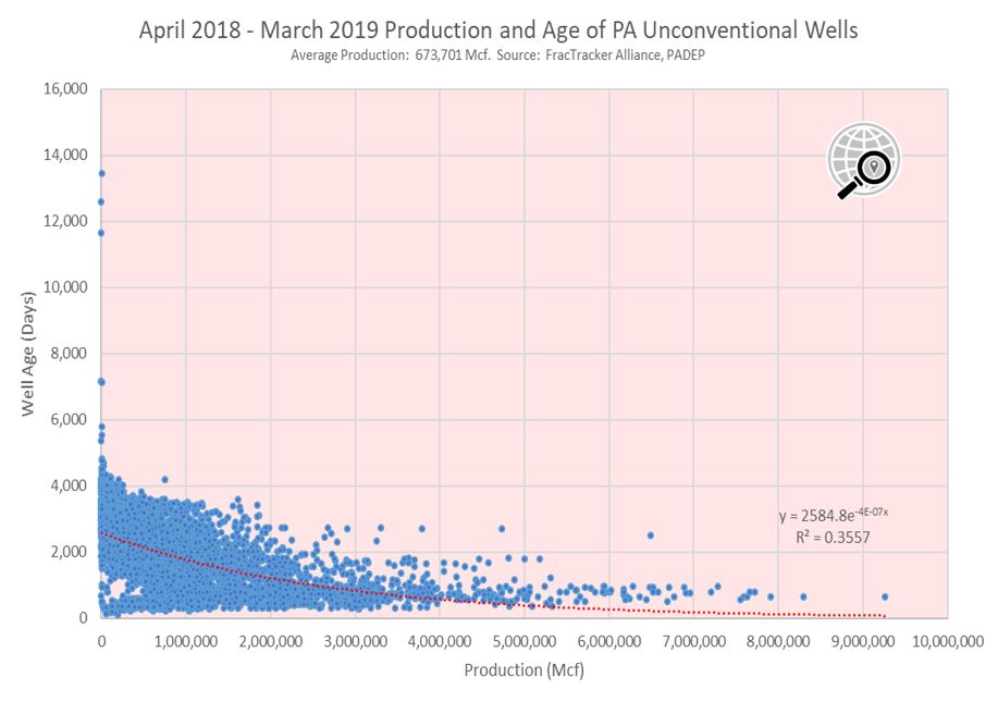
Figure 2 – 12 month gas production and age of well. Production is usually much higher during the earliest phases of the well’s production life.  This does not include wells that have been plugged or taken out of production.  Click on image for full-sized view.

In Figure 2, we look at the production of all unconventional wells in the state, expecting to see the highest production in younger wells. This mostly appears to be the case, but as mentioned above, there are also hot and cold spots with respect to production. A notable variable in this consideration is producing formation.

Since 93% (8,730 out of 9,404) of unconventional wells reporting gas production are in the Marcellus Shale Formation, the traditional hot spots in the northeastern and southwestern portions of the state heavily skew the overall totals in terms of both production and number of wells.  Other formations of note include the Onodaga Limestone (137 wells, 1.5% of total), Burket Member (117 wells, 1.2%), Genesee Formation (104 wells, 1.1%), and the Utica Shale (99 wells, 1.1%) (Figure 3).

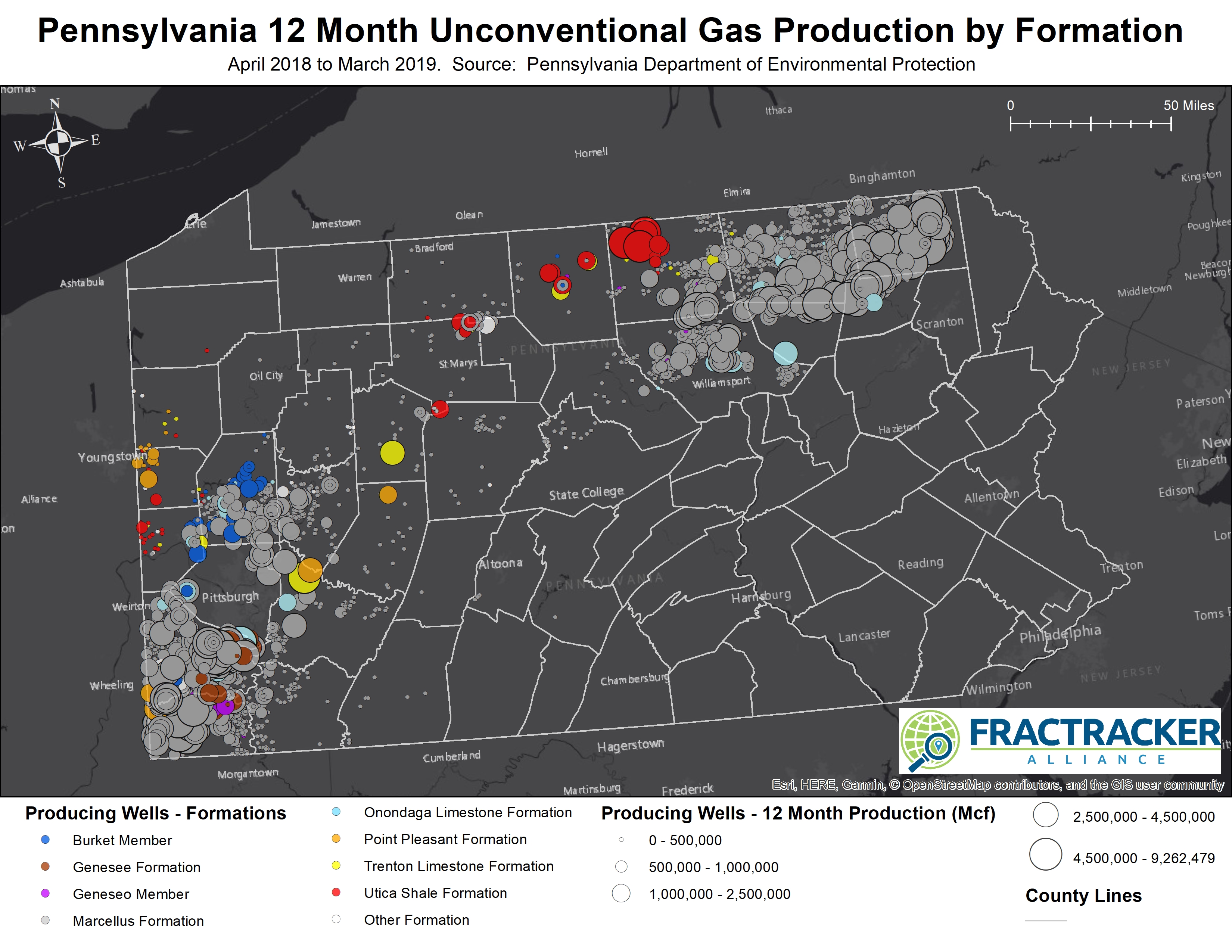
Figure 3 – Unconventional gas production over 12 months, showing formation. Click on image for full-sized view.

Drillers have been exploring some of these formations for decades. In fact, the oldest producing well that is currently classified as unconventional was 13,435 days old as of March 31, which works out to 36 years, 9 months, and 12 days.

However, this is fairly rare – only 384 (4%) of the 9,404 producing wells were more than 10 years old. 5,981 wells (64%) are between 5 and 10 years old, with the remaining 3,039 wells (32%) younger than 5 years old.

This does not take into account wells of any age that have been plugged or otherwise taken out of production.

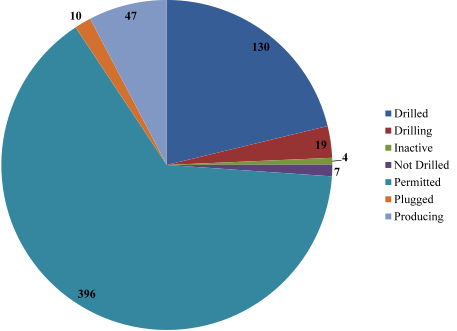
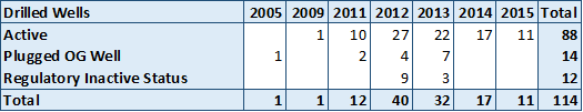
Age of Pennsylvania’s active wells
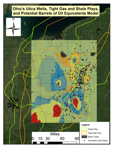
< 5 years old
5-10 years old
> 10 years old


Utica Shale

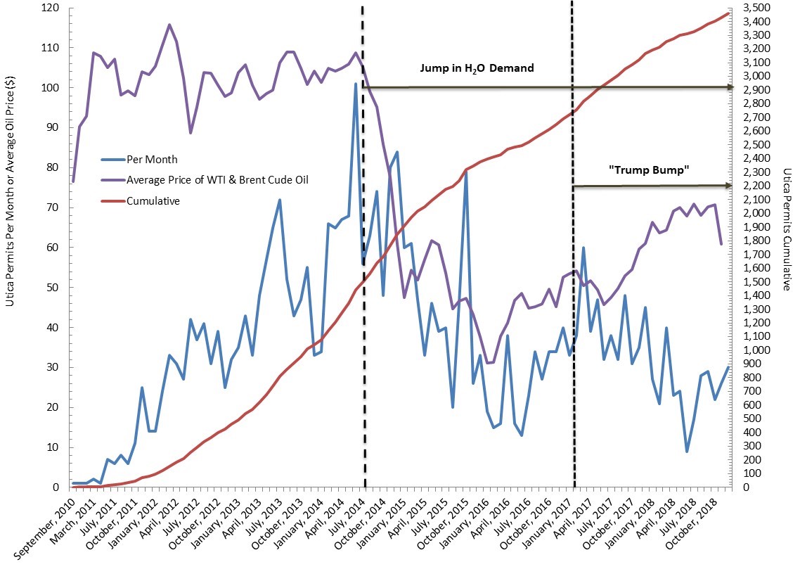
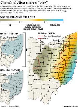
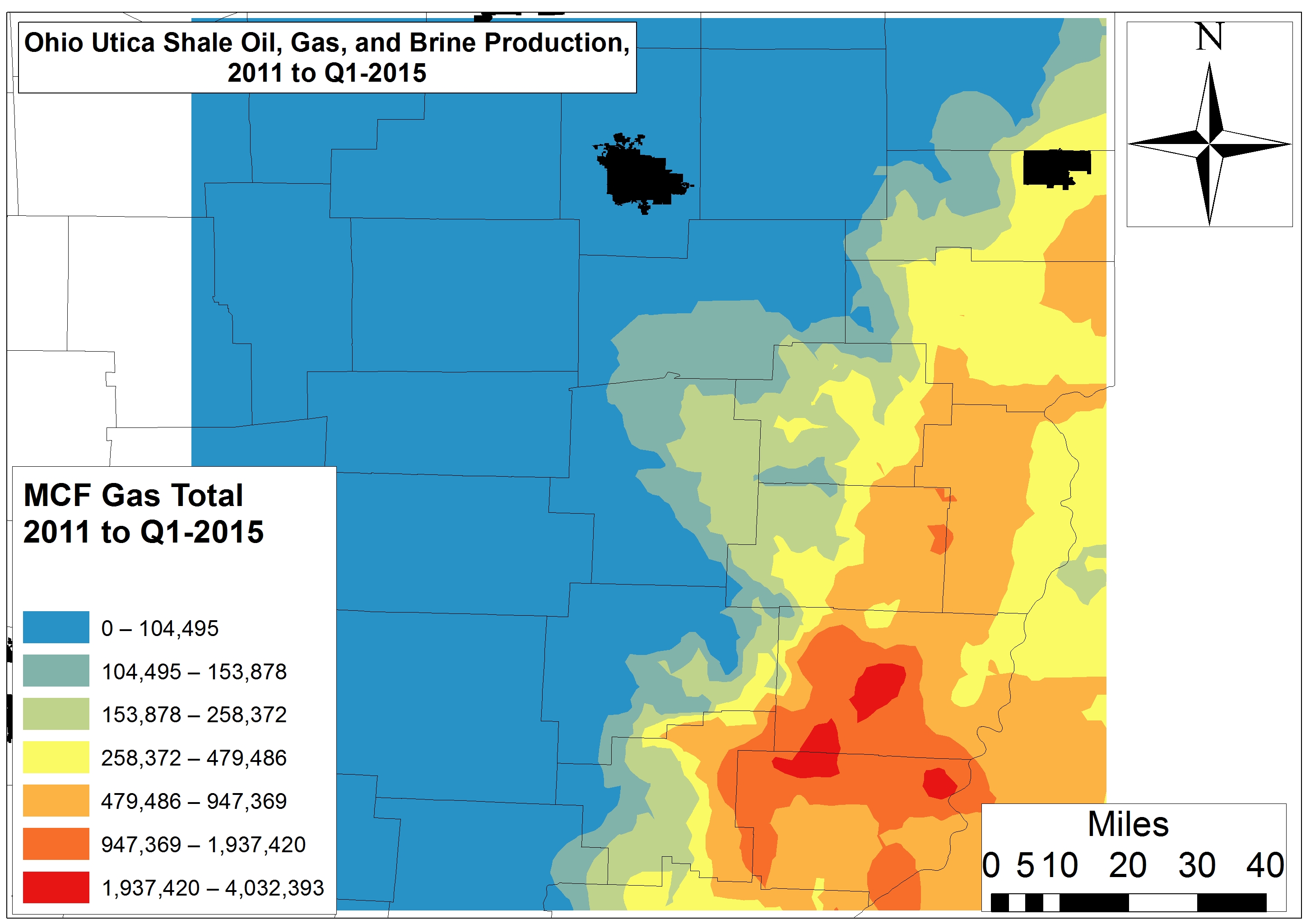
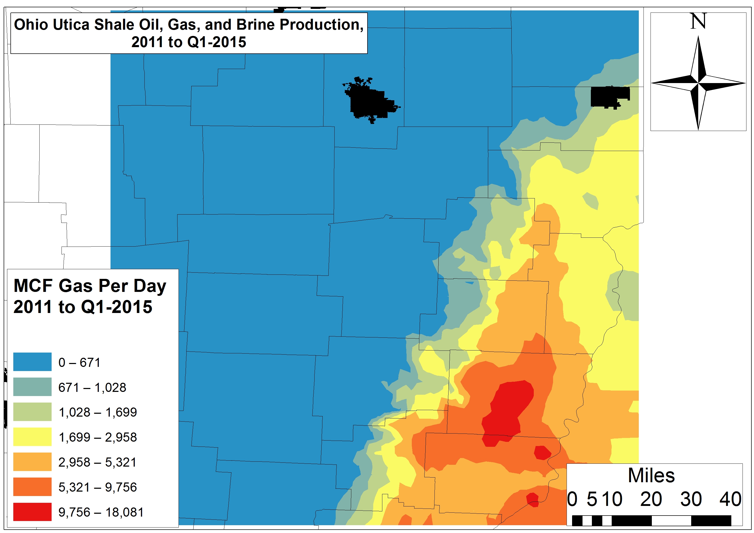
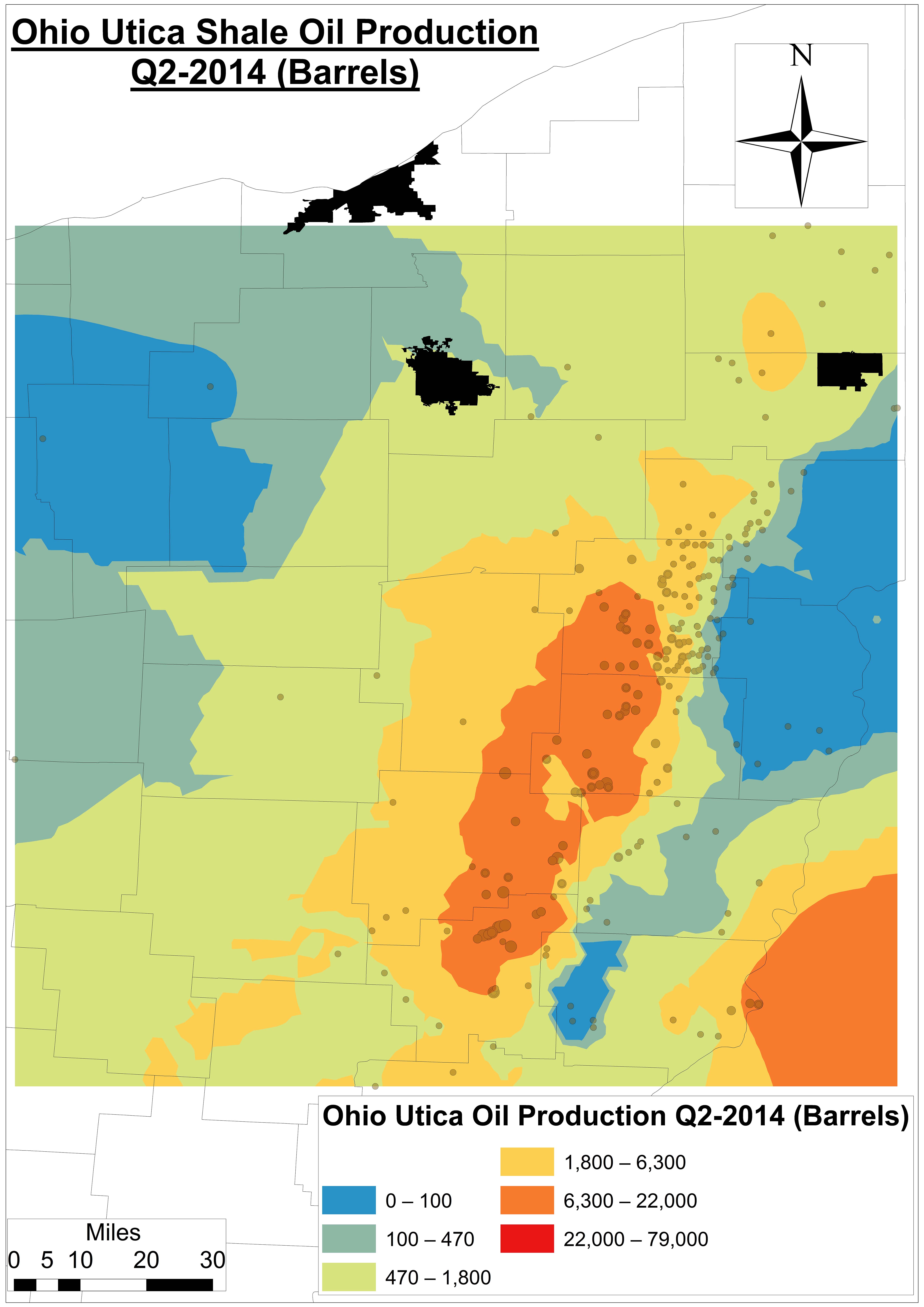
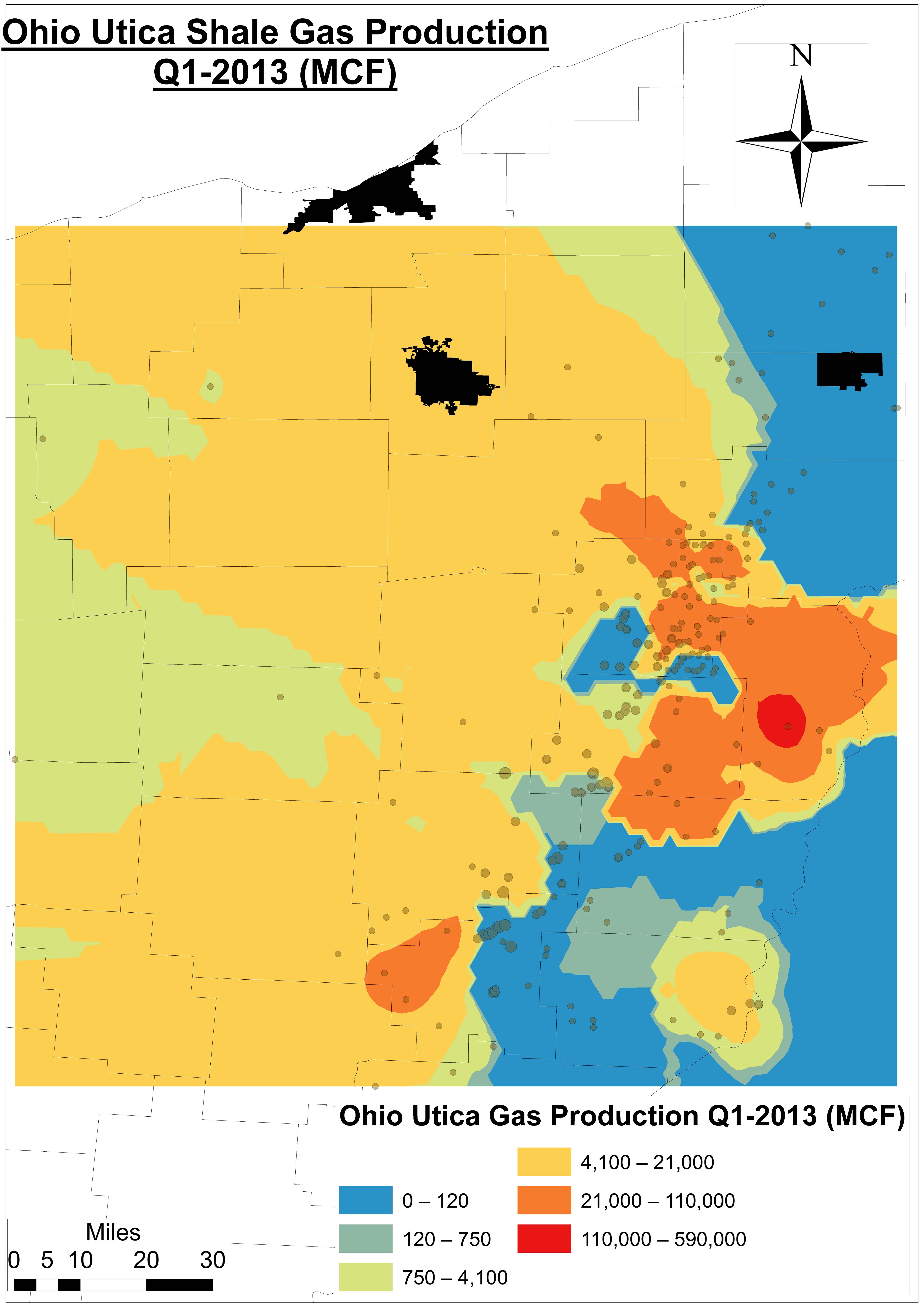
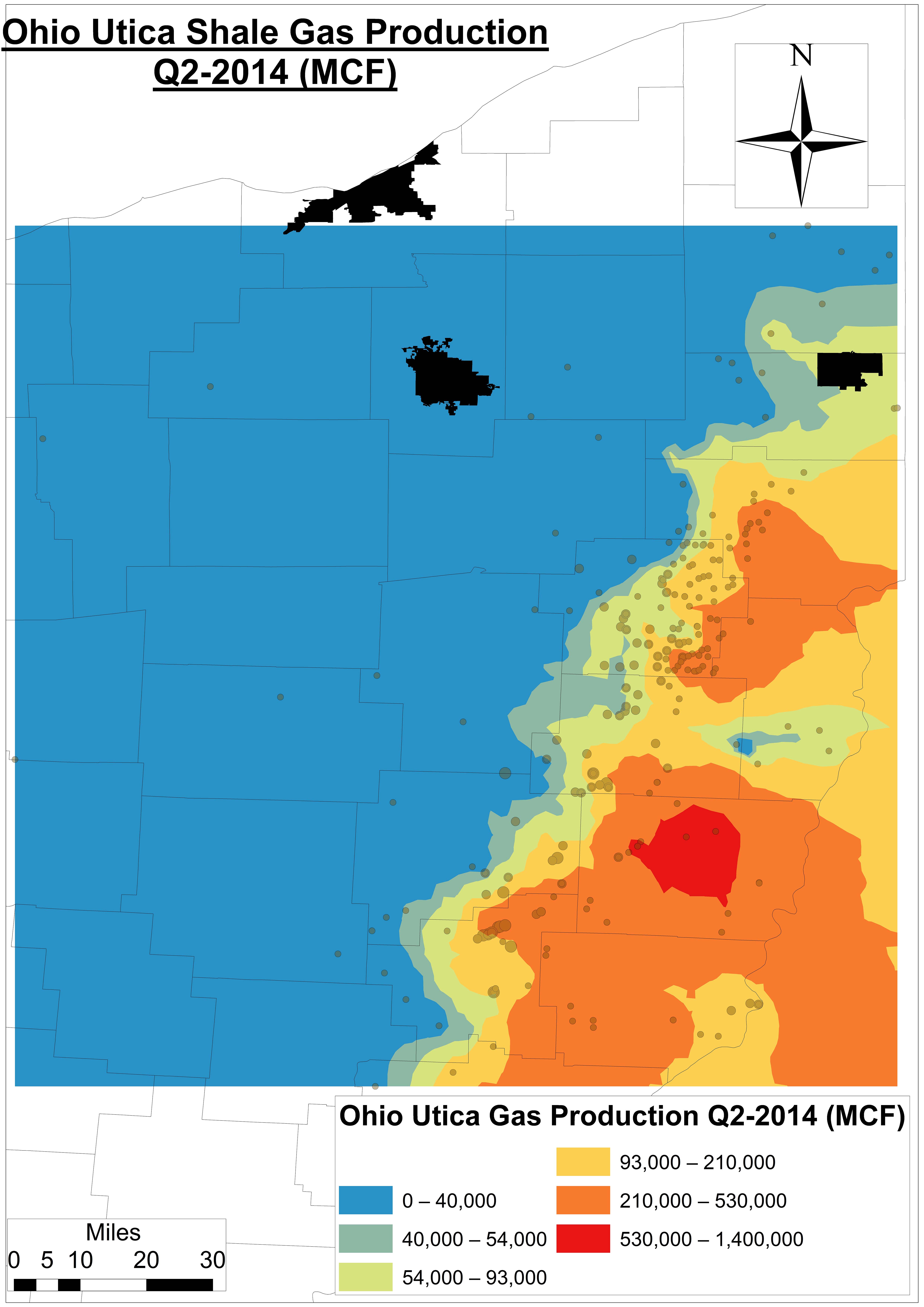
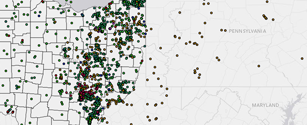
The Utica Shale is worth a special mention here for a couple of reasons.  First, we must acknowledge its prominence in neighboring Ohio, which has 2,160 permitted Utica wells to go with just 40 permitted Marcellus wells, the prevalence of the two plays seems to invert just as one passes over the state line. And yet, the most productive Utica wells are near the border with New York, not Ohio.

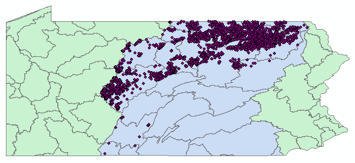
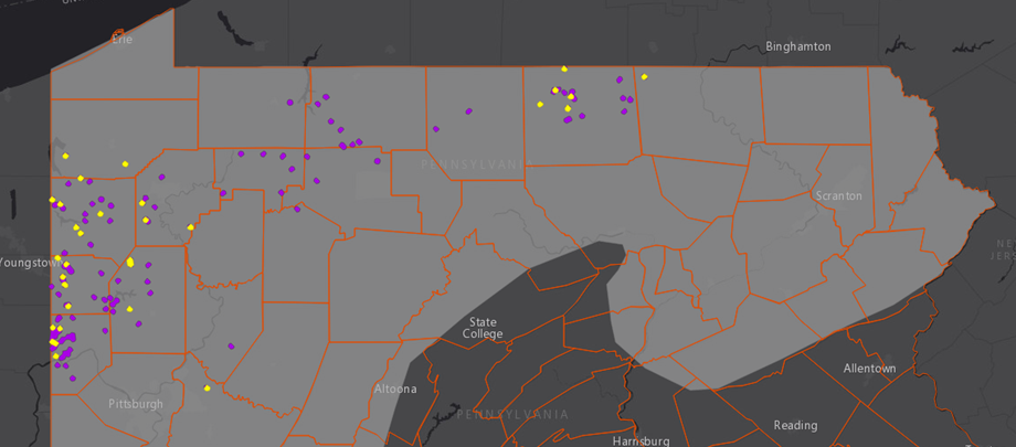
In fact, each of the top 11 producing Utica wells during the 12 month period were located in Tioga County.  It’s worth noting that these are all between one and two years old, which would have given the wells time to be drilled, fracked, and brought into production, while still being in the prime of their production life. Compared to the Marcellus, sample size quickly becomes an issue when analyzing the Utica in Pennsylvania (Figure 4).

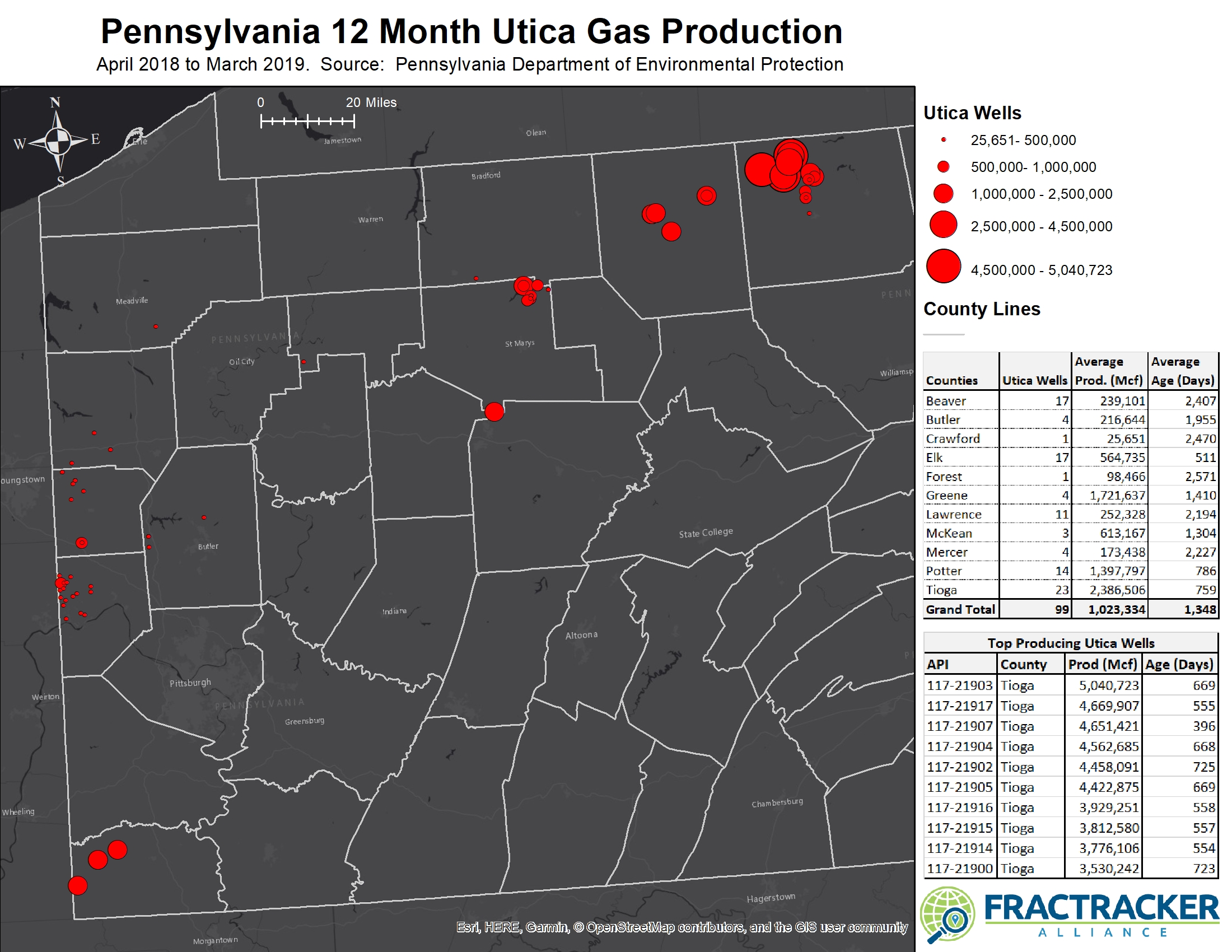
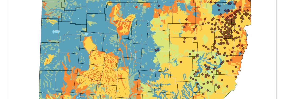
Figure 4 – Producing Utica wells in Pennsylvania. Note that the cluster of heavily producing wells in Tioga and Potter Counties near the New York border are mostly young wells where higher production would be expected.  Click on image for full sized view.

Second, portions of the Utica are known for their wet gas content, meaning that the gas has significant quantities of natural gas liquids (NGLs) including ethane, propane, and butane, which are gaseous at ambient temperatures but typically condensed into liquid form by oil and gas companies.  These are used for specialized fuels and petrochemical feedstocks, and are therefore more valuable than the methane in natural gas.

The production report does not capture the amount of NGLs in the gas, but a map from the Energy Information Administration shows the entire play, noting that the composition is dryer on the eastern portions of the play. In fact, a wet gas composition along the Ohio border might help to explain continued interest in what are otherwise well below average gas production results for Pennsylvania.

A Moving Target

It is difficult to predict where the industry will focus its attention in the coming months and years, but taking a look at production and formation data can give us a few clues.  Obviously, operators who found a particularly productive pocket of hydrocarbons are likely to keep drilling more holes in the ground in those areas until production is no longer profitable. Therefore, impacts to water, air, and nearby residents can be expected to continue in heavily drilled areas largely because the production level makes it attractive for drillers.

On the other hand, we should not assume that areas that are currently not productive are off the table for future consideration, either. Different formations are productive in different geographies, so a sweet spot for the Marcellus might be a dud in the Utica, or vice versa.

Finally, when comparing production, we must always take the age of the well into consideration, as all oil and gas wells can be expected to start off with a short period of very high production, followed by years of ever-diminishing returns throughout the expected 10 to 11 year lifecycle of the well. Because of this, what seems like a hotspot now may look below average in a similar analysis in three to four years, particularly in formations with relatively light drilling activity. This means that the top list of production by well could change over time, so be sure to check back in with FracTracker to see how events unfold.

By Matt Kelso, Manager of Data and Technology, FracTracker Alliance
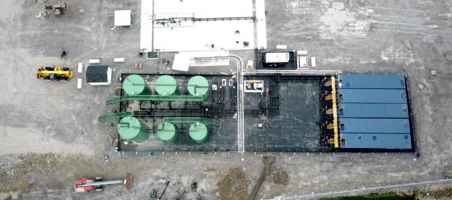
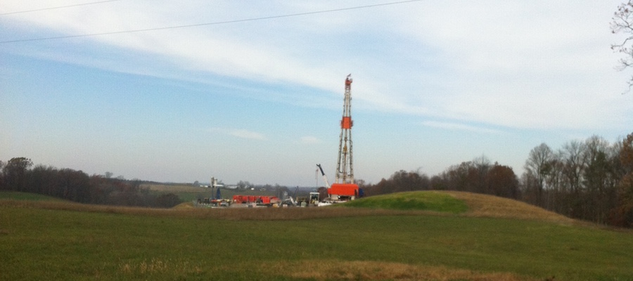
 

Bird's eye view of an injection well (oil and gas waste disposal)

A Disturbing Tale of Diminishing Returns in Ohio

Utica oil and gas production, Class II injection well volumes, and lateral length trends from 2010-2018

The US Energy Information Administration (EIA) recently announced that Ohio’s recoverable shale gas reserves have magically increased by 11,076 billion cubic feet (BCF). This increase ranks the Buckeye State in the top 5 for changes in recoverable shale natural gas reserves between 2016 and 2017 (pages 31- 32 here). After reading the predictable and superficial media coverage, we thought it was time to revisit the data to ask a pertinent question: What is the fracking industry costing Ohio?

Recent Shale Gas Trends in Ohio

According to the EIA’s report, Ohio currently sits at #7 on their list of proven reserves. It is estimated there are 27,021 BCF of shale gas beneath the state (Figure 1).

Graph of natural gas reserves in different states 2016-2017

Figure 1. Proven and change in proven natural gas reserves from 2016 to 2017 for the top 11 states and the Gulf of Mexico (calculated from EIA’s “U.S. Crude Oil and Natural Gas Proved Reserves, Year-End 2017”).

There are a few variations in the way the oil and gas industry defines proven reserves:

…an estimated quantity of all hydrocarbons statistically defined as crude oil or natural gas, which geological and engineering data demonstrate with reasonable certainty to be recoverable in future years from known reservoirs under existing economic and operating conditions. Reservoirs are considered proven if economic producibility is supported by either actual production or conclusive formation testing. – The Organization of Petroleum Exporting Countries

… the quantity of natural resources that a company reasonably expects to extract from a given formation… Proven reserves are classified as having a 90% or greater likelihood of being present and economically viable for extraction in current conditions… Proven reserves also take into account the current technology being used for extraction, regional regulations and market conditions as part of the estimation process. For this reason, proven reserves can seemingly take unexpected leaps and drops. Depending on the regional disclosure regulations, extraction companies might only disclose proven reserves even though they will have estimates for probable and possible reserves. – Investopedia

What’s missing from this picture?

Neither of the definitions above address the large volume of water or wastewater infrastructure required to tap into “proven reserves.” While compiling data for unconventional wells and injection wells, we noticed that the high-volume hydraulic fracturing (HVHF) industry is at a concerning crossroads. In terms of “energy return on energy invested,” HVHF is requiring more and more resources to stay afloat.

OH quarterly Utica oil & gas production along with quarterly Class II injection well volumes:

The map below shows oil and gas production from Utica wells (the primary form of shale gas drilling in Ohio). It also shows the volume of wastewater disposed in Class II salt water disposal injection wells.


 View map fullscreen | How FracTracker maps work

Publications like the aforementioned EIA article and language out of Columbus highlight the nominal increases in fracking productivity. They greatly diminish, or more often than not ignore, how resource demand and waste production are also increasing. The data speak to a story of diminishing returns – an industry requiring more resources to keep up gross production while simultaneously driving net production off a cliff (Figure 2).

Graph of Utica permits in Ohio on a cumulative and monthly basis along with the average price of West Texas Intermediate (WTI) and Brent Crude oil per barrel from September, 2010 to December, 2018

Figure 2. Number of Utica permits in Ohio on a cumulative and monthly basis along with the average price of West Texas Intermediate (WTI) and Brent Crude oil per barrel from September 2010 to December 2018

The Great Decoupling of New Year’s 2013

In the following analysis, we look at the declining efficiency of the HVHF industry throughout Ohio. The data spans the end of 2010 to middle of 2018. We worked with Columbus-area volunteer Gary Allison to conduct this analysis; without Gary’s help this work and resulting map, would not have been possible.

A little more than five years ago today, a significant shift took place in Ohio, as the number of producing gas wells increased while oil well numbers leveled off. The industry’s permitting high-water mark came in June of 2014 with 101 Utica permits that month (a level the industry hasn’t come close to since). The current six-month permitting average is 25 per month.

As the ball dropped in Times Square ringing in 2014, in Ohio, a decoupling between oil and gas wells was underway and continues to this day. The number of wells coming online annually increased by 229 oil wells and 414 gas wells.

Graph showing Number of producing oil and gas wells in Ohio’s Utica Shale Basin from 2011 to Q2-2018

Figure 3. Number of producing oil and gas wells in Ohio’s Utica Shale Basin from 2011 to Q2-2018

Graph of Producing oil and gas wells as a percentage of permitted wells in Ohio’s Utica Shale Basin from 2011 to Q2-2018

Figure 4. Producing oil and gas wells as a percentage of permitted wells in Ohio’s Utica Shale Basin from 2011 to Q2-2018

Permits

The ringing in of 2014 also saw an increase in the number of producing wells as a percentage of those permitted. In 2014, the general philosophy was that the HVHF industry needed to permit roughly 5.5 oil wells or 7 gas wells to generate one producing well. Since 2014, however, this ratio has dropped to 2.2 for oil and 1.4 for gas well permits.

Put another way, the industry’s ability to avoid dry wells has increased by 13% for oil and 18% for gas per year. As of Q2-2018, viable oil wells stood at 44% of permitted wells while viable gas wells amounted to 71% of the permitted inventory (Figure 4).

Production declines

from the top-left to the bottom-right

To understand how quickly production is declining in Ohio, we compiled annual (2011-2012) and quarterly (Q1-2013 to Q2-2018) production data from 2,064 unconventional laterals.

First, we present average data for the nine oldest wells with respect to oil and gas production on a per day basis (Note: Two of the nine wells we examined, the Geatches MAH 3H and Hosey POR 6H-X laterals, only produced in 2011-2012 when data was collected on an annual basis preventing their incorporation into Figures 6 and 7 belwo). From an oil perspective, these nine wells exhibited 44% declines from year 1 to years 2-3 and 91% declines by 2018 (Figure 5). With respect to natural gas, these nine wells exhibited 34% declines from year 1 to years 2-3 and 79% declines by 2018 (Figure 5).

Figure 5. Average daily oil and gas production decline curves for the above seven hydraulically fractured laterals in Ohio’s Utica Shale Basin, 2011 to Q2-2018

Four of the nine wells demonstrated 71% declines by the second and third years and nearly 98% declines by by Q2-2018 (Figure 6). These declines lend credence to recent headlines like Fracking’s Secret Problem—Oil Wells Aren’t Producing as Much as Forecast in the January 2nd issue of The Wall Street Journal. Four of the nine wells demonstrated 49% declines by the second and third years and nearly 81% declines by Q2-2018 (Figure 7).

Figure 6. Oil production decline curves for seven hydraulically fractured laterals in Ohio’s Utica Shale Basin from 2011 to Q2-2018

Figure 7. Natural gas production decline curves for seven hydraulically fractured laterals in Ohio’s Utica Shale Basin from 2011 to Q2-2018

Fracking waste, lateral length, and water demand

from bottom-left to the top-right

An analysis of fracking’s environmental and economic impact is incomplete if it ignores waste production and disposal. In Ohio, there are 226 active Class II Salt Water Disposal (SWD) wells. Why so many?

  1. Ohio’s Class II well inventory serves as the primary receptacle for HVHF liquid waste for Pennsylvania, West Virginia, and Ohio.
  2. The Class II network is situated in a crescent shape around the state’s unconventional wells. This expands the geographic impact of HVHF to counties like Ashtabula, Trumbull, and Portage to the northeast and Washington, Athens, and Muskingum to the south (Figure 8).
Map of Ohio showing cumulative production of unconventional wells and waste disposal volume of injection wells

Figure 8. Ohio’s unconventional gas laterals and Class II salt water disposal injection wells. Weighted by cumulative production and waste disposal volumes to Q3-2018.

Disposal Rates

We graphed average per well (barrels) and cumulative (million barrels) disposal rates from Q3-2010 to Q3-2018 for these wells. The data shows an average increase of 24,822 barrels (+1.05 million gallons) per well, each year.

That’s a 51% per year increase (Figure 9).

A deeper dive into the data reveals that the top 20 most active Class II wells are accepting more waste than ever before: an astounding annual per well increase of 728,811 barrels (+30.61 million gallons) or a 230% per year increase (Figure 10). This divergence resulted in the top 20 wells disposing of 4.95 times the statewide average between Q3-2010 and Q2-2013. They disposed 13.82 times the statewide average as recently as Q3-2018 (Figure 11).

All of this means that we are putting an increasing amount of pressure on fewer and fewer wells. The trickle out, down, and up of this dynamic will foist a myriad of environmental and economic costs to areas surrounding wells. As an example, the images below are injection wells currently under construction in Brookfield, Ohio, outside Warren and minutes from the Pennsylvania border.

More concerning is the fact that areas of Ohio that are injection well hotspots, like Warren, are proposing new fracking-friendly legislation. These disturbing bills would lubricate the wheels for continued expansion of fracking waste disposal and permitting. House bills 578 and 393 and Senate Bill 165 monetize and/or commodify fracking waste by giving townships a share of the revenue. Such bills “…would only incentivize communities to encourage more waste to come into their existing inventory of Class II… wells, creating yet another race to the bottom.” Co-sponsors of the bills include Democratic Reps. Michael O’Brien, Glenn Holms, John Patterson, and Craig Riefel.

Lateral Lengths

The above trends reflect an equally disturbing trend in lateral length. Ohio’s unconventional laterals are growing at a rate of 9.1 to 15.6%, depending on whether you buy that this trend is linear or exponential (Figure 12). This author believes the trend is exponential for the foreseeable future. Furthermore, it’s likely that “super laterals” in excess of 3-3.5 miles will have a profound impact on the trend. (See The Freshwater and Liquid Waste Impact of Unconventional Oil and Gas in Ohio and West Virginia.)

This lateral length increase substantially increases water demand per lateral. It also impacts Class II well disposal rates. The increase accounts for 76% of the former and 88% of the latter when graphed against each other (Figure 13).

Figure 12. Ohio Utica unconventional lateral length from Q3-2010 to Q4-2018

Figure 13. Ohio Utica unconventional water demand and Class II SWD injection well disposal volumes vs lateral length from Q3-2010 to Q4-2018.

Conclusion

This relationship between production, resource demand, and waste disposal rates should disturb policymakers, citizens, and the industry. One way to this problem is to more holistically price resource utilization (or stop oil and gas development entirely).

Unfortunately, states like Ohio are practically giving water away to the industry.

Politicians are constructing legislation that would unleash injection well expansion. This would allow disposal to proceed at rates that don’t address supply-side concerns. It’s startling that an industry and political landscape that puts such a premium on “market forces” is unwilling to address these trends with market mechanisms.

We will continue to monitor these trends and hope to spread these insights to states like Oklahoma and Texas in the future.

By Ted Auch, Great Lakes Program Coordinator, FracTracker Alliance – with invaluable data compilation assistance from Gary Allison


Data Downloads

FracTracker is a proponent of data transparency, and so we often share the data we use to construct our maps analyses. Click on the links below to download the data associated with the present analysis:

  • OH Utica laterals

    Ohio’s Utica HVHF laterals as of December 2018 in length (feet) (zip file)
  • Wastewater disposal volumes

    Inventory of volumes disposed on a quarterly basis from 2010 to Q3-2018 for all 223 active Class II Salt Water Disposal (SWD) Injection wells in Ohio (zip file)

The Curious Case of the Shrinking Utica Shale Play

Oil, Gas, and Brine Oh My!
By Ted Auch, Great Lakes Program Coordinator, FracTracker Alliance

It was just three years ago that the Ohio Geological Survey (OGS) and Department of Natural Resources (DNR) were proposing – and expanding – their bullish stance on the potential Utica Shale oil and gas production “play.” Back in April 2012 both agencies continue[d] to redraw their best guess, although as the Ohio Geological Survey’s Chief Larry Wickstrom cautioned, “It doesn’t mean anywhere you go in the core area that you will have a really successful well.”

What we found is that the OGS projections have not held up to their substantial claims. And here is why…

Background

The Geological Survey eventually parsed the Utica play into pieces:

  • a large oil component encompassing much of the central part of the state,
  • natural gas liquids from Ashtabula on the Pennsylvania border southwest to Muskingum, Guernsey, and Noble Counties, and
  • natural gas counties, primarily, along the Ohio River from Columbiana on the Pennsylvania-West Virginia border to Washington County in the Southeast quarter of the state.
Columbus Dispatch Utica Shale "play" map

Columbus Dispatch Utica Shale “play” map

Fast forward to the first quarter of 2015 and we have a very healthy dataset to begin to model and validate/refute these projections. Back in 2009 Wickstrom & Co. only had 53 Utica Shale laterals, while today Ohio is host to 962 laterals from which to draw our conclusions. The preponderance of producing wells are operated by Chesapeake (463), Gulfport (118), Antero Resources (62), Eclipse Resources (41), American Energy Utica (36), Consol (35), and R.E. Gas Development (34), with an additional 13 LLCs and 10 publicly traded companies accounting for the remaining 173 producing laterals. A further difference between the following analysis and the OGS one is that we looked at total production and how much oil and gas was produced on a per-day basis.

Analysis

Using an interpolative geostatistical technique known as Empirical Bayesian Kriging and the 962 lateral dataset, we modeled total and per day oil, gas, and brine production for Ohio’s Utica Shale between 2011 and Q1-2015 to determine if the aforementioned map redrawing holds up, is out-of-date, and/or is overly optimistic as is generally the case with initial O&G “moving target” projections.

Days of Activity & Brine Production

The most active regions of the Utica Shale for well pad activity has been much of Muskingum County and its border with Guernsey and Noble counties; laterals are in production every 1 in 2.1-3.4 days. Conversely, the least active wells have been drilled along the Harrison-Belmont border and the intersection between Harrison, Tuscarawas, and Guernsey counties.

Brine is a form of liquid drilling waste characterized by high salt loads and total dissolved solids. The laterals that have produced the most brine to date are located in a large section of Monroe County and at the intersection of Belmont, Monroe, and Noble counties, with total brine production amounting to 23,292 barrels or 734,000-978,000 gallons (Fig. 1).

Total Ohio Utica Shale Production Days 2011 to Q1-2015

Total Ohio Utica Shale Oil Production 2011 to Q1-2015

Total Ohio Utica Shale Gas Production 2011 to Q1-2015

Total Ohio Utica Shale Brine Production 2011 to Q1-2015

Figure 1. Total Ohio Utica Shale Oil, Gas, and Brine Production 2011 to Q1-2015

This area is also one of the top three regions of the state with respect to Class II Injection volumes; the other two high-brine production regions are Morrow and Portage counties to the west and southwest, respectively (Fig. 2).

Layout & Volume (2010 to Q1-2015, Gallons) of Ohio’s Active Class II Injection Wells

Figure 2. Layout & Volume (2010 to Q1-2015, Gallons) of Ohio’s Active Class II Injection Wells

However, on a per-day basis we are seeing quite a few inefficient laterals across the state, including Devon Energy’s Eichelberger and Richman Farms laterals in Ashland and Medina counties. Ashland and Medina are producing 230-270 barrels (8,453-9,923 gallons) of brine per day. In Carroll County, one of Chesapeake’s Trushell laterals tops the list for brine production at 1,843 barrels (67,730 gallons) per day. One of Gulfport’s Bolton laterals in Belmont County and EdgeMarc’s Merlin 10PPH in Washington County are generating 1,100-1,200 barrels (40,425-44,100 gallons) of brine per day.

Oil & Gas Production

Since the last time we modeled production the oil hotspots have shrunk. They have also become more discrete and migrated southward – all of this in contrast to the model proposed by the OGS in 2012. The areas of greatest productivity (i.e., >26,000 barrels of oil) are not the central part of the state, but rather Tuscarawas, Harrison, Guernsey, and Noble counties (Fig. 1). The intersection of Harrison, Tuscarawas, and Guernsey counties is where oil productivity per-day is highest – in the range of 300-630+ barrels (Fig. 3). The areas that the OGS proposed had the highest oil potential have produced <600 barrels total or <12 barrels per day.

Per Day Ohio Utica Shale Oil Production 2011 to Q1-2015

Per Day Ohio Utica Shale Gas Production 2011 to Q1-2015

Per Day Ohio Utica Shale Brine Production 2011 to Q1-2015

Figure 3. Per-Day Ohio Utica Shale Oil, Gas, and Brine Production 2011 to Q1-2015

The OGS natural gas region has proven to be another area of extremely low oil productivity.

Natural gas productivity in the Utica Shale is far less extensive than the OGS projected back in 2012. High gas production is restricted to discreet areas of Belmont and Monroe counties to the tune of 947,000-4.1 million Mcf to date – or 5,300-18,100 Mcf per day. While the OGS projected natural gas and natural gas liquid potential all the way from Medina to Fairfield and Perry counties, we found a precipitous drop-off in productivity in these counties to <1,028 Mcf per day (<155,000 Mcf total from 2011 to Q1-2015) or a mere 6-11% of the Belmont-Monroe sweet spot.

Conclusion: A Shrinking Utica Shale Play

Simply put, the OGS 2012 estimates:

  • Have not held up,
  • Are behind the times and unreliable with respect to citizens looking to guestimate potential royalties,
  • Were far too simplistic,
  • Mapped high-yield sections of the “play” as continuous when in fact productive zones are small and discrete,
  • Did not differentiate between per day and total productivity, and
  • Did not address brine waste.

These issues should be addressed by the OGS and ODNR on a more transparent and frequent basis. Combine this analysis with the disappointing returns Ohio’s 17 publicly traded drilling firms are delivering and one might conclude that the structural Utica Shale bubble is about to burst. However, we know that when all else fails these same firms can just “lever up,” like their Rocky Mountain brethren, to maintain or marginally increase production and shareholder happiness. Will these Red Queens of the O&G industry stay ahead of the Big Bank and Private Equity hounds on their trail?

Utica Drilling in Pennsylvania

In Pennsylvania, the vast majority of unconventional oil and gas activity is focused on the Marcellus Shale formation, a Devonian period deposit of black shale with a high hydrocarbon content, which requires horizontal drilling and large scale hydraulic fracturing to produce enough oil and gas to make the drilling economically viable.  This formation was created about 390 million years ago, when organic-rich deposits accumulated in what is now the Appalachian Mountains, but was at that time a shallow sea.  Down below the base of the Marcellus lies the Utica Shale, an Ordovician period formation, with almost the same geographic extent as the Marcellus, but the deposits were placed there about 65 million years earlier.


Utica permits and violations in Pennsylvania. Click here to access the legend and other map tools.

In neighboring Ohio, it is the Utica that gets most of the attention, with 937 permitted wells, as opposed to just 20 for the Marcellus.  In Pennsylvania, the reverse is true:  there are 16,110 permitted Marcellus wells, but only 279 permits for Utica wells.  Part of the reason for this is because the subsurface characteristics of these formations vary widely, especially in terms of thickness and depth.  With changes in depth come changes in temperature and pressure, which are key criteria in hydrocarbon formation.  In other words, the same formation that produces considerable quantities of gas and valuable liquid hydrocarbons in eastern Ohio may be economically unviable just a county or two over in western Pennsylvania.

Utica shale permits, drilled wells, violations, and violations per well for Pennsylvania, through June 19, 2015.

Utica shale permits, drilled wells, violations, and violations per well for Pennsylvania, through June 19, 2015.

Utica drilling permits have been issued in 19 different counties in Pennsylvania, with wells having been drilled in 15 of those.  The violations per well (VpW) score for Utica wells in the Keystone State is 0.9, meaning that there are nine violations issued for every 10 wells that have been drilled.  It is worth noting, however, that only 36 of the 114 drilled wells have received violations, meaning that some wells have been cited on multiple occasions.

Of particular note is Bradford county, the site of only one Utica well, but 19 items on the compliance report.  The problematic Bayles 1 well was run by three different operators before being permanently plugged.  This well also has two “Drill Deeper” permits, and as a result, it is likely that the first six violations assessed to this well were issued before it was associated with the Utica Shale, as they precede the most recent spud date for the well in June, 2005.  Most of the violations for this well seem to be for pit violations and discharges to the ground and nearby stream.

Wells drilled into the Utica Formation in Pennsylvania, by year and current status.

Wells drilled into the Utica Formation in Pennsylvania, by year and current status.

In terms of drilling activity, it appears to have peaked in 2012, calling into question whether the industry considers the formation to be economically viable in Pennsylvania.  Of the 28 wells drilled since the beginning of 2014, Tioga County has seen the most activity with 11 wells drilled, followed by five wells in Butler County, then three in Lawrence County.  If we think of drilling activity as a sort of positive feedback from the industry – meaning that they like what they see and want to keep exploring – then only Tioga County seems to be holding the attention of the various operators who have been active in the Utica Shale.  Given the Utica activity in Ohio, one might have thought that counties on the western edge of the state – especially Beaver, Lawrence, and Mercer – would have shown the most promise, but this appears not to be the case.

The Water-Energy Nexus in Ohio, Part II

OH Utica Production, Water Usage, and Waste Disposal by County
Part II of a Multi-part Series
By Ted Auch, Great Lakes Program Coordinator, FracTracker Alliance

In this part of our ongoing “Water-Energy Nexus” series focusing on Water and Water Use, we are looking at how counties in Ohio differ between how much oil and gas are produced, as well as the amount of water used and waste produced. This analysis also highlights how the OH DNR’s initial Utica projections differ dramatically from the current state of affairs. In the first article in this series, we conducted an analysis of OH’s water-energy nexus showing that Utica wells are using an ave. of 5 million gallons/well. As lateral well lengths increase, so does water use. In this analysis we demonstrate that:

  1. Drillers have to use more water, at higher pressures, to extract the same unit of oil or gas that they did years ago,
  2. Where production is relatively high, water usage is lower,
  3. As fracking operations move to the perimeter of a marginally productive play – and smaller LLCs and MLPs become a larger component of the landscape – operators are finding minimal returns on $6-8 million in well pad development costs,
  4. Market forces and Muskingum Watershed Conservancy District (MWCD) policy has allowed industry to exploit OH’s freshwater resources at bargain basement prices relative to commonly agreed upon water pricing schemes.

At current prices1, the shale gas industry is allocating < 0.27% of total well pad costs to current – and growing – freshwater requirements. It stands to reason that this multi-part series could be a jumping off point for a more holistic discussion of how we price our “endless” freshwater resources here in OH.

In an effort to better understand the inter-county differences in water usage, waste production, and hydrocarbon productivity across OH’s 19 Utica Shale counties we compiled a data-set for 500+ Utica wells which was previously used to look at differenced in these metrics across the state’s primary industry players. The results from Table 1 below are discussed in detail in the subsequent sections.

Table 1. Hydrocarbon production totals and per day values with top three producers in bold

County

# Wells

Total

Per Day

Oil

Gas

Brine

Production

Days

Oil

Gas

Brine

Ashland

1

0

0

23,598

102

0

0

231

Belmont

32

55,017

39,564,446

450,134

4,667

20

8,578

125

Carroll

256

3,715,771

121,812,758

2,432,022

66,935

67

2,092

58

Columbiana

26

165,316

9,759,353

189,140

6,093

20

2,178

65

Coshocton

1

949

0

23,953

66

14

0

363

Guernsey

29

726,149

7,495,066

275,617

7,060

147

1,413

49

Harrison

74

2,200,863

31,256,851

1,082,239

17,335

136

1,840

118

Jefferson

14

8,396

9,102,302

79,428

2,819

2

2,447

147

Knox

1

0

0

9,078

44

0

0

206

Mahoning

3

2,562

0

4,124

287

9

0

14

Medina

1

0

0

20,217

75

0

0

270

Monroe

12

28,683

13,077,480

165,424

2,045

22

7,348

130

Muskingum

1

18,298

89,689

14,073

455

40

197

31

Noble

39

1,326,326

18,251,742

390,791

7,731

268

3,379

267

Portage

2

2,369

75,749

10,442

245

19

168

228

Stark

1

17,271

166,592

14,285

602

29

277

24

Trumbull

8

48,802

742,164

127,222

1,320

36

566

100

Tuscarawas

1

9,219

77,234

2,117

369

25

209

6

Washington

3

18,976

372,885

67,768

368

59

1,268

192

Production

Total

It will come as no surprise to the reader that OH’s Utica oil and gas production is being led by Carroll County, followed distantly by Harrison, Noble, Belmont, Guernsey and Columbiana counties. Carroll has produced 3.7 million barrels of oil to date, while the latter have combined to produce an additional 4.5 million barrels. Carroll wells have been in production for nearly 67,000 days2, while the aforementioned county wells have been producing for 42,886 days. The remaining counties are home to 49 wells that have been in production for nearly 8,800 days or 7% of total production days in Ohio.

Combined with the state’s remaining 49 producing wells spread across 13 counties, OH’s Utica Shale has produced 8.3 million barrels of oil as well as 251,844,311 Mcf3 of natural gas and 5.4 million barrels of brine. Oil and natural gas together have an estimated value of $2.99 billion ($213 million per quarter)4 assuming average oil and natural gas prices of $96 per barrel and $8.67 per Mcf during the current period of production (2011 to Q2-2014), respectively.

Potential Revenue at Different Severance Tax Rates:

  • Current production tax, 0.5-0.8%: $19 million ($1.4 Million Per Quarter (MPQ). At this rate it would take the oil and gas industry 35 years to generate the $4.6 billion in tax revenue they proposed would be generated by 2020.
  • Proposed, 1% gas and 4% oil: At Governor Kasich’s proposed tax rate, $2.99 billion translates into $54 million ($3.9 MPQ). It would still take 21 years to return the aforementioned $4.6 billion to the state’s coffers.
  • Proposed, 5-7%: Even at the proposed rate of 5-7% by Policy Matters OH and northeastern OH Democrats, the industry would only have generated $179 million ($12.8 MPQ) to date. It would take 11 years to generate the remaining $4.42 billion in tax revenue promised by OH Oil and Gas Association’s (OOGA) partners at IHS “Energy Oil & Gas Industry Solutions” (NYSE: IHS).5

The bottom-line is that a production tax of 11-25% or more ($24-53 MPQ) would be necessary to generate the kind of tax revenue proposed by the end of 2020. This type of O&G taxation regime is employed in the states of Alaska and Oklahoma.

From an outreach and monitoring perspective, effects on air and water quality are two of the biggest gaps in our understanding of shale gas from a socioeconomic, health, and environmental perspective. Pulling out a mere 1% from any of these tax regimes would generate what we’ll call an “Environmental Monitoring Fee.” Available monitoring funds would range between $194,261 and $1.8 million ($16 million at 55%). These monies would be used to purchase 2-21 mobile air quality devices and 10-97 stream quantity/quality gauges to be deployed throughout the state’s primary shale counties to fill in the aforementioned data gaps.

Per-Day Production

On a per-day oil production basis, Belmont and Columbiana (20 barrels per day (BPD)) are overshadowed by Washington (59 BPD) and Muskingum (40 BPD) counties’ four giant Utica wells. Carroll is able to maintain such a high level of production relative to the other 15 counties by shear volume of producing wells; Noble (268 BPD), Guernsey (147 BPD), and Harrison (136 BPD) counties exceed Carroll’s production on a per-day basis. The bottom of the league table includes three oil-free wells in Ashland, Knox, and Medina, as well as seventeen <10 BPD wells in Jefferson and Mahoning counties.

With respect to natural gas, Harrison (1,840 Mcf per day (MPD)) and Guernsey counties are replaced by Monroe (7,348 MPD) and Jefferson (2,447 MPD) counties’ 26 Utica wells. The range of production rates for natural gas is represented by the king of natural gas producers, Belmont County, producing 8,578 MPD on the high end and Mahoning and Coshocton counties in addition to the aforementioned oil dry counties on the low end. Four of the five oil- or gas-dry counties produce the least amount of brine each day (BrPD). Coshocton, Medina, and Noble county Utica wells are currently generating 267-363 barrels of BrPD, with an additional seven counties generating 100-200 BrPD. Only four counties – 1.2% of OH Utica wells – are home to unconventional wells that generate ≤ 30 BrPD.

Water Usage

Freshwater is needed for the hydraulic fracturing process during well stimulation. For counties where we had compiled a respectable sample size we found that Monroe and Noble counties are home to the Utica wells requiring the greatest amount of freshwater to obtain acceptable levels of productivity (Figure 1). Monroe and Noble wells are using 10.6 and 8.8 million gallons (MGs) of water per well. Coshocton is home to a well that required 10.8 MGs, while Muskingum and Washington counties are home to wells that have utilized 10.2 and 9.5 MGs, respectively. Belmont, Guernsey, and Harrison reflect the current average state of freshwater usage by the Utica Shale industry in OH, with average requirements of 6.4, 6.9, and 7.2 MGs per well. Wells in eight other counties have used an average of 3.8 (Mahoning) to 5.4 MGs (Tuscarawas). The counties of Ashland, Knox, and Medina are home to wells requiring the least amount of freshwater in the range of 2.2-2.9 MGs. Overall freshwater demand on a per well basis is increasing by 220,500-333,300 gallons per quarter in Ohio with percent recycled water actually declining by 00.54% from an already trivial average of 6-7% in 2011 (Figure 2).

Water and production (Mcf and barrels of oil per day) in OH’s Utica Shale.

Figure 1. Average water usage (gallons) per Utica well by county

Average water usage (gallons) on a per well basis by OH’s Utica Shale industry, shown quarterly between Q3-2010 and Q2-2014.

Figure 2. Average water usage (gallons) on per well basis by OH Utica Shale industry, shown quarterly between Q3-2010 & Q2-2014.

Belmont County’s 30+ Utica wells are the least efficient with respect to oil recovery relative to freshwater requirements, averaging 7,190 gallons of water per gallon of oil (Figure 3). A distant second is Jefferson County’s 14 wells, which have required on average 3,205 gallons of water per gallon of oil. Columbiana’s 26 Utica wells are in third place requiring 1,093 gallons of freshwater. Coshocton, Mahoning, Monroe, and Portage counties are home to wells requiring 146-473 gallons for each gallon of oil produced.

Belmont County’s 14 Utica wells are the least efficient with respect to natural gas recovery relative to freshwater requirements (Figure 4). They average 1,306 gallons of water per Mcf. A distant second is Carroll County’s 250+ wells, which have injected 520 gallons of water 7,000+ feet below the earth’s service to produce a single Mcf of natural gas. Muskingum’s Utica well and Noble County’s 39 wells are the only other wells requiring more than 100 gallons of freshwater per Mcf. The remaining nine counties’ wells require 15-92 gallons of water to produce an Mcf of natural gas.

Water and production (Mcf and barrels of oil per day) in OH’s Utica Shale – Average Water Usage Per Unit of Oil Produced (Gallons of Water Per Gallon of Oil).

Figure 3. Average water usage (gallons) per unit of oil (gallons) produced across 19 Ohio Utica counties

Water and production (Mcf and barrels of oil per day) in OH’s Utica Shale – Average Water Usage Per Unit of Gas Produced (Gallons of Water Per MCF of Gas)

Figure 4. Average water usage (gallons) per unit of gas produced (Mcf) across 19 Ohio Utica counties

Waste Production

The aforementioned Jefferson wells are the least efficient with respect to waste vs. product produced. Jefferson wells are generating 12,728 gallons of brine per gallon of oil (Figure 5).6 Wells from this county are followed distantly by the 32 Belmont and 26 Columbiana county wells, which are generating 5,830 and 3,976 gallons of brine per unit of oil.5 The remaining counties (for which we have data) are using 8-927 gallons of brine per unit of oil; six counties’ wells are generating <38 gallons of brine per gallon of oil.

Water and production (Mcf and barrels of oil per day) in OH’s Utica Shale – Average Brine Production Per Unit of Oil Produced (Gallons of Brine Per Gallon of Oil)

Figure 5. Average brine production (gallons) per gallon of oil produced per day across 19 Ohio Utica Counties

The average Utica well in OH is generating 820 gallons of fracking waste per unit of product produced. Across all OH Utica wells, an average of 0.078 gallons of brine is being generated for every gallon of freshwater used. This figure amounts to a current total of 233.9 MGs of brine waste produce statewide. Over the next five years this trend will result in the generation of one billion gallons (BGs) of brine waste and 12.8 BGs of freshwater required in OH. Put another way…

233.9 MGs is equivalent to the annual waste production of 5.2 million Ohioans – or 45% of the state’s current population. 

Due to the low costs incurred by industry when they choose to dispose of their fracking waste in OH, drillers will have only to incur $100 million over the next five years to pay for the injection of the above 1.0 BGs of brine. Ohioans, however, will pay at least $1.5 billion in the same time period to dispose of their municipal solid waste. The average fee to dispose of every ton of waste is $32, which means that the $100 million figure is at the very least $33.5 million – and as much as $250.6 million – less than we should expect industry should be paying to offset the costs.

Environmental Accounting

In summary, there are two ways to look at the potential “energy revolution” that is shale gas:

  1. Using the same traditional supply-side economics metrics we have used in the past (e.g., globalization, Efficient Market Hypothesis, Trickle Down Economics, Bubbles Don’t Exist) to socialize long-term externalities and privatize short-term windfall profits, or
  2. We can begin to incorporate into the national dialogue issues pertaining to watershed resilience, ecosystem services, and the more nuanced valuation of our ecosystems via Ecological Economics.

The latter will require a more real-time and granular understanding of water resource utilization and fracking waste production at the watershed and regional scale, especially as it relates to headline production and the often-trumpeted job generating numbers.

We hope to shed further light on this new “environmental accounting” as it relates to more thorough and responsible energy development policy at the state, federal, and global levels. The life cycle costs of shale gas drilling have all too often been ignored and can’t be if we are to generate the types of energy our country demands while also stewarding our ecosystems. As Mark Twain is reported to have said “Whiskey is for drinking; water is for fighting over.” In order to avoid such a battle over the water-energy nexus in the long run it is imperative that we price in the shale gas industry’s water-use footprint in the near term. As we have demonstrated so far with this series this issue is far from settled here in OH and as they say so goes Ohio so goes the nation!

A Moving Target

ODNR projection map of potential Utica productivity from Spring, 2012

Figure 6. ODNR projection map of potential Utica productivity from spring 2012

OH’s Department of Natural Resources (ODNR) originally claimed a big red – and nearly continuous – blob of Utica productivity existed. The projection originally stretched from Ashtabula and Trumbull counties south-southwest to Tuscarawas, Guernsey, and Coshocton along the Appalachian Plateau (See Figure 6).

However, our analysis demonstrates that (Figures 7 and 8):

  1. This is a rapidly moving target,
  2. The big red blob isn’t as big – or continuous – as once projected, and
  3. It might not even include many of the counties once thought to be the heart of the OH Utica shale play.

This last point is important because counties, families, investors, and outside interests were developing investment and/or savings strategies based on this map and a 30+ year timeframe – neither of which may be even remotely close according to our model.

An Ohio Utica Shale oil production model for Q1-2013 using an interpolative Geostatistical technique called Empirical Bayesian Kriging.

Figure 7a. An Ohio Utica Shale oil production model using Kriging6 for Q1-2013

An Ohio Utica Shale oil production model for Q2-2014 using an interpolative Geostatistical technique called Empirical Bayesian Kriging.

Figure 7b. An Ohio Utica Shale oil production model using Kriging for Q2-2014

An Ohio Utica Shale gas production model for Q1-2013 using an interpolative Geostatistical technique called Empirical Bayesian Kriging.

Figure 8a. An Ohio Utica Shale gas production model using Kriging for Q1-2013

An Ohio Utica Shale gas production model for Q2-2014 using an interpolative Geostatistical technique called Empirical Bayesian Kriging.

Figure 8b. An Ohio Utica Shale gas production model using Kriging for Q2-2014


Footnotes

  1. $4.25 per 1,000 gallons, which is the current going rate for freshwater at OH’s MWCD New Philadelphia headquarters, is 4.7-8.2 times less than residential water costs at the city level according to Global Water Intelligence.
  2. Carroll County wells have seen days in production jump from 36-62 days in 2011-2012 to 68-78 in 2014 across 256 producing wells as of Q2-2014.
  3. One Mcf is a unit of measurement for natural gas referring to 1,000 cubic feet, which is approximately enough gas to run an American household (e.g. heat, water heater, cooking) for four days.
  4. Assuming average oil and natural gas prices of $96 per barrel and $8.67 per Mcf during the current period of production (2011 to Q2-2014), respectively
  5. IHS’ share price has increased by $1.7 per month since publishing a report about the potential of US shale gas as a job creator and revenue generator
  6. On a per-API# basis or even regional basis we have not found drilling muds data. We do have it – and are in the process of making sense of it – at the Solid Waste District level.
  7. An interpolative Geostatistical technique formally called Empirical Bayesian Kriging.

Ohio Production and Injection Well Firms Map

Our latest Ohio-focused map shows the many companies involved in directional drilling in the state and the contact information for these firms.

Layer Descriptions

1. UNIVERSAL WELL SERVICES

Universal Well Services Inc. is a major firm involved in all manner of directional drilling services with an office in Wooster, OH, one in Allen, KY, six in Pennsylvania, six in Texas, and one in West Virginia

2. LLC & MLP’s

This is an inventory of 410 Ohio directional drilling affiliated LLC and MLP firms and contact information. Seventy-eight percent of these firms are domiciled in Ohio. The other primary states that house these firms are Pennsylvania (22), Texas (23), and West Virginia (9). The Economist wrote of these types of firms:

The move away from the C corporation began in earnest in 1975. Wyoming, that vibrant business hub, adopted a new entity structure, the limited-liability company (LLC). Imported from Panama, it provided the tax treatment of a partnership while preserving the corporate protection from individual liability for company debts and litigation. Other states followed in adopting the model. Businesses were quick to see the advantages. The various new types of firm that have risen in the wake of the LLC… make similar use of partnership structures. They have tended to be industry- or sector-specific, at least to begin with. The energy business has a lot of MLPs not only because it needs capital but because it is an easy place to set them up: since 1987, tax law has allowed “mineral or natural resource” companies to operate as listed partnerships, while withholding that privilege from others. But as with other pass-through structures, the constraints are being lowered and circumvented.

3. DRILLING FIRMS

This is an inventory of 393 Ohio Department of Natural Resources permitted directional and injection drilling firms with single locations and their contact information. Seventy-six percent of these firms are domiciled in Ohio with the other primary states of incorporation being Pennsylvania (15), Texas (14), Michigan (11), and West Virginia (9). Only 3 of these firms listed in the Ohio RBDMS Microsoft Access Database contained correct contact information or addresses. According to ODNR staff – and primary FOIA contact:

… it looks like the [active drillers] list [doesn’t contain] much information on the companies in general…We have mailing information for the operating companies, but a lot of the time they subcontract out to get their drillers. We do not require the information of the drillers they contract.

4. ADDITIONAL DRILLERS

This is an inventory of the 40 known locations for six firms permitted to drill in Ohio. The same lack of contact and address data for these firms were true for this data. The primary firms are Butch’s Rathole and Nomac Drilling Corporation. Given that the ODNR RBDMS does not indicate the actual location from which these companies migrated into the Ohio shale industry we decided to include all known locations for these firms.

5. CANADIAN FIRMS

This is an inventory of the 14 known locations for the 5 Canadian drilling firms permitted in Ohio. The primary firm is Savannah Drilling, which is composed of 10 locations across Alberta and Saskatchewan.

6. AMERICAN SUPPORTING CO.

This is an inventory of 1,837 Ohio energy firms operating in the Utica and Marcellus shale or servicing it in a secondary or tertiary fashion. Seventy-five percent (1,386) of these firms are domiciled in Ohio with secondary hotspots in Texas (76), West Virginia (65), Pennsylvania (49), Michigan (34), Colorado (27), Illinois (22), Oklahoma (21), California (16), New York and New Jersey (27), Kentucky (14).

7. ADDITIONAL SUPPORTING CO.

This shows an inventory of 10 Ohio energy firms operating in the Utica and Marcellus shale or servicing it in a secondary or tertiary fashion extracted from the ODNR RBDMS that did not contain locational or contact information.

8. CANADIAN SUPPORTING CO.

This is an inventory of 5 (1 company Mar Oil Company was not found) Canadian energy firms operating in the Utica and Marcellus shale or servicing it in a secondary or tertiary fashion.

9. BRINE HAULERS

This is an inventory of 505 ODNR permitted brine haulers active in the transport and disposal of hydraulic fracturing waste either via injection or waste landfill disposal. Seventy-six percent of these firms are domiciled in Ohio with the primary cities being Zanesville (18), Cambridge, Wooster, and Millersburg (12 each), Canton and Marietta (11 each), Columbus (9), Jefferson (9), Logan (8), and North Canton and Newark (7 each). Pennsylvania and West Virginia are home to 84 and 32 brine haulers, respectively.

Ohio’s Shale Gas Waste Disposal Network Map Now Online

By Ted Auch, Ohio Program Coordinator, FracTracker Alliance

A complete inventory of Ohio’s Active Class II Injection Wells, as well as Ohio Department of Natural Resources certified Underground Injection Control (UIC) certified transporters, is now available in map form on FracTracker.org (See embedded map below). There is an interest in mapping Ohio’s waste facility network for many reasons; in addition to concerns regarding the spreading of waste on roads, problems with Class II Injection Wells in Youngstown are forcing the state to turn to secondary disposal options.

Shale Gas Waste Disposal Network


To view the map’s full set of controls, including legend, please click on the “fullscreen” button on the map.

Map Layers

In addition to the Class II waste injection wells, the map includes Ohio disposal wells designated for Enhanced Oil Recovery (129), Annular Disposal (82), Salt Water Disposal (221), Temporarily Abandoned Annular Disposal (1,987), and Class II Salt Mining (57).

Active Class II’s have quarter-mile buffering increments from 0.10 to 1.5 miles.On average, Ohio’s active Class II wells are 4,434±2,032 feet deep, with a maximum depth of 13,727 feet. There is a total of 793,734 linear feet worth of active Class II wells throughout the state. Utilizing capacity estimates from current Class II fracking waste well permits in Portage County, Ohio, the state’s active Class II’s are capable of accepting 34.6-97.2 million gallons of fracking waste. However, if we include the state’s aforementioned Class II’s that are not currently being utilized for fracking waste disposal, this capacity estimate jumps to 510.9-1,437.4 million gallons of fracking waste. Such volumes would profoundly affect surface water volumes and flows (i.e., headwater streams and vernal pools), aquifer and sub-surface water chemistry, and the types of issues facing California. [1]

At the present time Ohio’s Utica wells are utilizing 4.2-4.5 million gallons of water and 206,837-261,907 gallons of brine per well with an average of 1.96 barrels of brine produced per barrel of oil. To date Ohio’s 213 reported producing wells have utilized 949 million gallons of water and 681,789 gallons of brine. If the state’s remaining 481 permitted Utica wells produce and utilize water at a similar rate The Utica Play would utilize approximately 3.03 billion gallons of water and produce 113 million gallons of brine all of which would require additional Ohio Class II Injection Well capacity requiring the state to repurpose the existing stock to handle this sizeable increase in fracking fluids, drill cuttings and muds, and related oilfield fluids. Thus, FracTracker felt the need to begin to map the state’s non-shale gas Class II Injection Wells.

The map also shows the locations of current natural gas compressor stations and underground storage tanks, along with the state’s hazardous waste and orphaned landfills. These sites were included in response to the Ohio EPA’s recent advisory suggesting waste landfill facilities begin accepting drill cuttings, drilling muds and frac sands, and related oilfield fluids [1,2].

We also present Ohio’s network of Bulk Transporters, which are charged with transporting related materials.

Acknowledgements

This is an original map from The FracTracker Alliance and was constructed with the assistance of Ohio State University graduate student, Caleb Gallemore, and a selection of students from his GIS Class “Elements of Cartography: Serving the Community through cartography.” It was made possible by information from Bulk Transporter Magazine. [3]


References

[1]  Staff. (2013, May 14). Will Ohio’s Landfills Become a Dumping Ground for Radioactive Fracking Waste? EcoWatch. Read>

[2] See our recent post: Ohio’s Waste Not, Want Not!

[3] Who in their words “is the information source for liquid and dry bulk logistics industry. Written for bulk shippers, transporters, and storage operators, BT is dedicated to providing the latest information on regulations, technological developments, logistics management, and hazardous materials safety. For over 65 years, BT has been a trusted source of information for the bulk logistics industry.”

Land-Use Change, the Utica Shale, and the Loss of Ecosystem Services

By Ted Auch, PhD – Ohio Program Coordinator, FracTracker Alliance

In Ohio, Utica Well pads range in size from 5-15 acres. (Estimates for pipeline and retention ponds are unavailable.) That figure gives us the chance to estimate how hydraulic fracturing influenced changes to land-use, ecosystem services, plant productivity, and soil carbon loss.

Working with Caleb Gallemore and his Ohio State University GIS class, we created a data set that estimated the percent cover for each well pad prior to drilling using the USGS and Department of Interior’s 2006 National Land Cover Database (NLCD, 2006) [1].

Figure 1. Ohio’s original vegetation cover and Utica Well permits as of April 30th, 2013

Figure 1. Ohio’s original vegetation cover and Utica Well permits as of April 30, 2013

Accordingly, the state was and is dominated by:

  • mixed oak (from 12,038 mi2 pre-settlement to 7,911 mi2 today) to the east and
  • maple-beech-birch (from 13,917 mi2 pre-settlement to 2,521 mi2 today) to the west stretching into the southeast and northwest corner of Ohio.

During pre-settlement times additional dominant forest types included:

Since industrialization:

  • The faster growing elm-ash-cottonwood has arisen as a sub-dominant forest type currently comprising 1,237 mi2.
  • Additional sub-dominant forest types comprising 100-140 mi2 of Ohio’s land area include aspen-birch (134 mi2), white-red-jack pine (124 mi2), and loblolly-shortleaf pine (108 mi2).

Our results suggest the average amount of deciduous forest [2] disturbed – as a percent of total well pad area – by well pad establishment is 9.8 ± 5.5% per well pad with a range of 4.7% in Stark and Holmes Counties and a high of 24% in Monroe County (Figure 2). With respect to pasture and crop displacement the average is 11.7 and 10.7% per well pad, respectively, with significantly higher between-county variability for crop cover (±5.5% Vs ±3.6%).

Figure 2. Percent Cover across Ohio’s 269 Utica Well Pads assuming an average area of 7.75 acres and the National Land Cover Database 2006 (NLCD 2006) as a proxy for previous land-use.

Figure 2. Percent Cover across Ohio’s 269 Utica Well Pads assuming an average area of 7.75 acres and the National Land Cover Database 2006 (NLCD 2006) as a proxy for previous land-use. – Click to enlarge

Converting this data into ecosystem services requires certain assumptions about plant growth, soil organic matter content, and soil compaction utilizing Natural Resource Conservation Service (NRCS) soil data to model the latter two and established peer-reviewed estimates for plant pattern and process (Follett, Kimble, & Lal, 2000; Lobell et al., 2002; Valentine et al., 2012). The basics of this analysis – assuming subsurface soils are 25% more compact and contain 45% less organic matter than the surface 12-13 inches (Needelman et al., 1999) – demonstrated that well pad establishment has displaced approximately 28,205 tons of surface and 78,348 tons of subsurface soil carbon [3] for a total of 106,554 tons of carbon equivalent to 389,986 tons of CO2.

Additionally, the displacement and/or removal of vegetation – assuming the average Ohio forest is 40-80 years old [4] – has resulted in the annual loss of 1,050, 6,516, and 9,461 tons of crop, pasture, and forest carbon production, respectively. This is equal to 17,027 tons of carbon or 62,319 tons of CO2, which when added to the aforementioned soil loss is equivalent to the CO2 footprint of 25,198 Ohioans [5].

Over the life of these three ecosystem types, well pad establishment displaces 1,021,619 tons of carbon. This equates to 3.74 million tons of CO2 or 230,034 Ohioans, which is roughly 9,000 less people than reside in Akron and Warren combined. Another way way to frame this figure is that it would be equivalent to the eightieth largest US city between Henderson, NV and Scottsdale, AZ.

At CO2’s current valuation this Ohio Utica well pad “carbon displacement” is roughly $18.71 million. However, if we assume this is at the lower end of reasonable CO2 estimates and that a range of $10-75 dollars is more indicative of carbon’s price, then we estimate the value of well pad displaced carbon is more like $41.29-309.68 million.

The true value of Utica well pad carbon displacement is somewhere in this range and entirely dependent on your belief in the feasibility of valuing CO2 emissions. However, these estimates do point to some of the externalities associated with Utica Shale development currently ignored by industry lobbyists and political advocates. There is far more work to be done as it relates to understanding well pads’ influence on ecosystem services, crop productivity, and local hydrology; this is simply an attempt to begin quantifying such effects.


References

Follett, R F, Kimble, J M, & Lal, R. (2000). The Potential of U.S. Grazing Lands to Sequester Carbon and Mitigate the Greenhouse Effect. Boca Raton, FL: CRC Press LLC.

Fry, J, Xian, G, Jin, S, Dewitz, J, Homer, C, Yang, L, . . . Wickham, J. (2011). Completion of the 2006 National Land Cover Database for the Conterminous United States. PE&RS, 77(9), 858-864.

Lobell, D B, Hicke, J A, Asner, G P, Field, C B, Tucker, C J, & Los, S O. (2002). Satellite estimates of productivity and light use efficiency in United States agriculture, 1982-98. Global Change Biology, 8(8), 722-735.

Needelman, B A, Wander, M M, Bollero, G A, Boast, C W, Sims, G K, & Bullock, D G. (1999). Interaction of Tillage and Soil Texture Biologically Active Soil Organic Matter in Illinois. Soil Science Society of America Journal, 63(5), 1326-1334.

Valentine, J, Clifton-Brown, J, Hastings, A, Robson, P, Allison, G, & Smith, P. (2012). Food vs. Fuel: The use of land for lignocellulosic next generation energy crops to minimize competition with primary food production. Global Change Biology Bioenergy, 4(1), 1-19.


Footnotes

[1] The NLCD estimates land cover using sixteen classes at a 98 foot spatial resolution applied to 2006 Landsat satellite data or 4-5 years prior to the first Ohio Utica permit in September, 2010 (Fry et al., 2011)

[2] Primary tree species include red and sugar maple, red and white oak, white ash, black cherry, American beech, hickory, and tulip poplar according to the most recent USFS Forest Inventory Analysis “Ohio Forests 2006”.

[3] Along with roughly 6,536 tons of soil nitrogen assuming an Ohio soil Carbon-To-Nitrogen ratio of 14.6.

[4] Utilizing the USFS’s Forest Inventory and Analysis EVALIDator Version 1.5.1.04 tool we determined that 62% of Ohio’s oak-hickory, maple-beech-birch, elm-ash-cottonwood, and oak-pine forest types, which account for 94% of the state’s forest area, are 40-80 years old.

[5] Assuming 17.3-18.6 tons of CO2 per capita based on Oak Ridge National Laboratory’s Carbon Dioxide Information Analysis Center as cited by the World Bank.

A Year in the Life of Ohio’s Utica Play

The Ohio Utica play has taken off in the last calendar year, jumping from 160 permitted wells as of March 2012 to 453 since then. This equates to 1.24 permitted wells per day. (Note: The state’s less exploited Marcellus shale had 13 permitted wells a year ago with an increase of 7 since then.) A year ago Ohio was home to 50 “drilled” wells and is now home to an additional 80 “drilled” wells (Figure 1). Meanwhile 0.65% and 1.14% of permitted wells are what Ohio Department of Natural Resources (ODNR) calls “Inactive” or “Not Drilled” with the latter being relatively similar a year ago vs. today with 3 and 4 “Not Drilled” wells, respectively. According to the latest ODNR data 54 Utica wells were permitted as of 4/1/2012 vs. 342 since then. Plugged wells constitute 1.63% of all Ohio Utica wells although the industry appears to be increasing efficiency with respect to plugging having experienced 7 “Plugged” wells as of 4/1/2012 and only 3 since. Conversely, wells that are “Producing” have declined from 25.63% (41 “Producing” wells) of all permitted wells to 1.32% (6 “Producing” wells) of all permitted wells since then with the latest reported producing well being a Mountaineer Keystone well in Windham Township, Portage County.

The permitting process has continued along its exponential path since permitting began September 28, 2010 (Figure 2). The gross average number of permitted Ohio Utica wells per month in the last five months is 39 with a total of 195 permitted since November 2012. The quarterly permit average has increased by an order of magnitude of 4.2 permits per month between September 2010 and 2011 to 39 per month since September 2012. In recent months Washington county was added to the list of Ohio counties home to Utica hydraulic fracturing permits, while Carroll remains the state with the most Utica permits followed by Harrison, Columbiana, Guernsey, and Jefferson/Noble with the average number of Utica well permits across the 22 counties home to at least one permit being 28 per county with six counties above and sixteen below this mean (Figure 3). In the last year the four counties that have entered the Utica conversation are Trumbull, neighboring Holmes and Wayne, and Washington, with 4, 3, 1, and 1 Utica permit as of April 1st, respectively. Meanwhile five other counties have seen no increase in Utica permits including Muskingum, Knox, Ashland, Geauga, and Medina. Conversely Belmont County has seen a 21-fold increase in Utica well permits followed distantly by Harrison, Guernsey, Noble, and Coshocton counties all of which have experienced ≥5-fold increases.

The average number of people per Utica well across the aforementioned 22 counties is 31,808, while the average number of wells per square mile is 0.066. The range is quite broad for both variables ranging from 0.0018 wells per square mile in Wayne – home to the Wayne National Forest – to 0.59 wells per square mile in Carroll County, with the one recent Washington County well placing it 13th out of 22 counties. The inverse is the case for people per well with Medina County, home to the highest number of people relative to Utica well permits with 172,332 people per well (vs. 124-563 people per well in Carroll, Harrison, Noble, and Monroe counties).  Since last we conducted this type of analysis in late January the valuation of Ohio’s major Utica players has actually increased by 11.7%. This is a particularly complex situation considering that Atlas Noble the owner of 6 Utica wells has actually gone private for a variety of reasons and Chesapeake Energy has ousted its CEO Aubrey McClendon due to “philosophical differences and a pending SEC investigation. Meanwhile, Wall Street-types:

… expect well results to vary greatly, given 2012 drilling activity across many fringe areas of the play. We believe weak results from other operators are likely to validate that Gulfport remains the most exposed operator. Source

Additionally, the repeated delay in 2012 production numbers scheduled for the 1st of April is creating layer upon layer of uncertainty leaving everyone guessing and relying on 2011 production numbers. This leaves public sentiment worried about the unsustainability, uncoordinated, and unbalanced nature of both Ohio’s regulatory framework and highly Utica exposed and/or leveraged balance sheets. Meanwhile Wall Street analysts are contemplating whether market forces, expectations, reality, or collusion is to blame. Our current model of potential Utica production in the form of barrels of oil equivalent speaks to small and discrete highly productive zones in Belmont, Noble, Guernsey, Morgan, and Muskingum counties, rather than the originally estimated zones of highest production in Carroll and Columbiana. An additional hotspot appears to be located in Fairfield, Perry, and Hocking counties. However, due to insufficient data quantity, quality, and methodology, and transparency from ODNR and industry, the opportunities to conduct such exercises are still accompanied by substantial uncertainty in the form of high signal-to-noise resulting from scant and unreliable data. The hope, herein and on Wall Street, is that ODNR and industry will begin to make their production data available in real-time.

This is an especially important consideration given that the aforementioned regulatory environment here in Ohio – as well as the relatively generous severance taxing system[1] – has reached a point that even industry/supply-side think tanks like The Fraser Institute in Canada have determined “the extent of investment barriers (based on All-Inclusive Composite Index values)” are as good as they are ever going to get; Ohio trails only Mississippi in a global investment barrier ranking of 146 countries, US states, and Canadian provinces. Furthermore, in one year the conditions for doing largely hydrocarbon-related business in Ohio improved so much between 2010 and 2011 that Ohio jumped up the league tables from 12th to 2nd, according to the institute’s 2011 “Global Petroleum Survey.” This loosening of regulations, combined with decreasing data quality and availability, is the primary concern of The FracTracker Alliance in Ohio.

Utica Permit activity by status to April 1, 2013

Figure 1: Utica Permit activity by status to April 1, 2013

Figure 2. Cumulative and Per Month Utica Permits to September 2010 through March 2013

Figure 2. Cumulative and Per Month Utica Permits to September 2010 through March 2013

Figure 3. Utica Permit Count by County from September 28, 2010 to April 1, 2013

Figure 3. Utica Permit Count by County from September 28, 2010 to April 1, 2013

Figure 4. Utica Permits Per Square Mile and People Per Well by County from September 28, 2010 to April 1, 2013

Figure 4. Utica Permits Per Square Mile and People Per Well by County from September 28, 2010 to April 1, 2013

(Note: This model was constructing utilizing the Geostatistical Analyst Tools “Empirical Bayesian Kriging” tool in ArcGIS)

Figure 5. A map of the current Ohio Shale and Tight Gas Plays, hydraulic fracturing permits in Ohio as of 4/1/2013, and a generalized model of potential production from with light green representing 20 Barrels of Oil Equivalent (BOE) and red approximately 10,000 BOE

Table 1. Distribution of Ohio Utica Shale wells across companies (#, %), Date of First Permit (DFP), and the valuation of the publicly funded companies at their DFP at the close of business 4/9/2013.


Company Valuation

Company

#

%

DFP

Share Price DFP

Share Price 4/9/2013

% Change

Anadarko

12

0.019

09/07/2011

69.88

86.70

1.241

Antero

21

0.034

03/23/2012

Atlas Noble††

6

0.010

09/24/2012

31.14

Carrizo

2

0.003

07/26/2012

24.02

26.26

1.093

Chesapeake Energy

389

0.626

12/23/2010

25.61

19.99

0.781

Chevron Appalachia

2

0.003

07/31/2012

109.58

118.71

1.083

Consol Energy

25

0.040

06/17/2011

45.86

33.85

0.738

Devon Energy

13

0.021

11/02/2011

65.46

55.28

0.844

Eclipse Resources

1

0.002

12/21/2012

Enervest

16

0.026

06/30/2011

9.37

8.79

0.938

EQT

3

0.005

09/13/2012

57.76

69.59

1.205

Gulfport Energy

46

0.074

02/28/2012

35.49

48.09

1.355

Halcon

2

0.003

11/02/2012

5.003

7.69

1.537

Hall Drilling

1

0.002

09/17/2012

Hess Ohio

24

0.039

09/28/2010

53.63

73.50

1.371

HG Energy

16

0.026

09/14/2011

Hilcorp Energy

3

0.005

12/14/2012

Mountaineer Keystone

7

0.011

07/13/2012

PDC Energy

9

0.014

05/25/2012

25.67

47.59

1.854

R E Gas Development

13

0.021

03/19/2012

Sierra Resources

3

0.005

07/02/2012

SWEPI

1

0.002

06/20/2012

XTO Energy

5

0.008

04/09/2012

0.28

0.01

0.036

BP

1

0.002

03/20/2013

613

1.083

DFP = Date of First Permit; “—“ not a publicly traded company

†† Atlas Noble has since gone private

Corporations that have reported production numbers as of this post: 1) Anadarko – 3, 2) Chesapeake – 14, 3) Consol Energy – 1, 4) Enervest and PDC Energy – 2, 5) Gulfport – 10, R E Gas Development – 4.


[1] Ernst & Young in a 2011 report found that Ohio’s hydrocarbon taxing rates were the most favorable of the eight states they investigated with a total state and local tax of 1.8% vs. 10.9-11.0% in neighboring West Virginia and Oklahoma, respectively. The average across the seven other states was 9.2% or 5.12 times that of The Buckeye State.

Unconventional oil and gas wells in the Chesapeake Basin

A Fresh Opportunity in the FRESHER Act

By Tanya Dierolf, Choose Clean Water Coalition

Love him or hate him, there’s no arguing that Stephen Colbert can grab a headline. Recently he’s had a lot to say about environmental protection, energy and water. Last week he reported on the Pegasus Pipeline Spill in Arkansas and reminded us that what’s “out of sight” and “out of mind” might still be in our drinking water. Those of us in Pennsylvania familiar with Talisman Terry have yet to forget his exposé on the children’s coloring book that attempts to teach kids about hydraulic fracturing through the expertise of a friendly Frackasaurus. This leaves me wondering if Colbert might ask Congressman Matt Cartwright about his legislative attempts to apply stricter federal protections to oil and gas development when the Pennsylvania Congressman appears on Stephen’s “Better Know a District” segment in early May.

In March 2013, Congressman Cartwright (PA-17) introduced the “Focused Reduction of Effluence and Stormwater runoff through Hydrofracking Environmental Regulation Act” or FRESHER act. Because of expanding development of oil and gas wells in Pennsylvania and exploration, construction, and operations in almost 30 other states, Mr. Cartwright introduced legislation aimed at fixing a federal Clean Water Act loophole to control stormwater runoff from for oil and gas operations. Under the Clean Water Act, industrial facilities are required to obtain a permit to discharge stormwater from their sites and develop “Stormwater Pollution Prevention Plans” if disturbing more than one acre of land. However, Congress exempted oil and gas operations from both of these requirements. By closing the loophole, the FRESHER Act would provide for stronger oversight as both regulators and the public would be aware of industry plans to control pollution. The bill would also require a federal study of stormwater impacts in areas that might be contaminated by stormwater runoff pollution from oil and gas operations.

Chesapeake Bay Watershed

Many of us working in the Chesapeake Bay watershed are often asked about the impacts that increasing natural gas activity may have on our local waters and the larger Chesapeake Bay cleanup. Considering the ongoing challenges we have with sediment impacts to our local waterways in Pennsylvania and West Virginia and the pollution limits we now have in place to bring the Bay back to health, many are asking how we quantify these impacts. In addition to increased sediment pollution largely carried by stormwater runoff, others are also asking what impact a change in our land use might have as we convert farm fields and forests to well pads. Furthermore, many are asking about roads and pipelines and cumulative impacts. All good questions – and these are just related to natural gas development and its relationship to existing pollution limits and cleanup plans. There are a host of additional questions being asked about drinking water, emissions, groundwater contamination, methane migration, and health and safety.

Mapping a Better Picture

Unconventional oil and gas wells in the Chesapeake Basin

Unconventional Oil and Gas Wells in PA’s portion of the Chesapeake Bay Watershed
Click here to view dynamic, PA map of unconventional wells

To get an idea of the impacts of the oil and gas industry in the Chesapeake Bay watershed, we turned to our colleagues at the FracTracker Alliance. FracTracker is committed to working with partners – citizens, organizations, and institutions – in a quest for objective, helpful information to perpetuate awareness and support actions that protect public health, the environment, and socioeconomic well-being. FracTracker collects, interprets and shares data through a website and mapping tool. When it came time to understand impacts, we asked for and received some numbers.

In the portion of Pennsylvania that has waterways draining to the Chesapeake Bay, there have been 5,137 oil and gas wells drilled since 2005*. This number includes both conventional and unconventional wells and vertical and horizontal wells (see map on right). Pennsylvania defines an “unconventional well” as one that is drilled into an unconventional formation, which is defined as a geologic shale formation between the base of the Elk Sandstone or its geologic equivalent where natural gas generally cannot be produced except by horizontal or vertical well bores stimulated by hydraulic fracturing. In short, the definition does include wells drilled within the Marcellus Shale formation. We are continuing to work with FracTracker to obtain similar information on West Virginia.

In Practice

I don’t want to leave the impression that oil and gas development, specifically gas development because of hydraulic fracturing, is an unregulated industry. For example, Pennsylvania already requires erosion & sediment permits for activities involving earth disturbance activities over five acres. I’m also not attempting to get into the patchwork of state-by-state regulations of the oil and gas industry, but Congressman Cartwright’s legislation would ensure that oil and gas companies have stormwater-related permits and pollution prevention plans in place prior to well pad development. The lack of oversight and permitting represents a significant threat to our waterways in places without adequate accountability mechanisms. It’s a fresh opportunity to address an ongoing challenge. We hope Mr. Colbert might just ask Mr. Cartwright about his efforts as we get to know PA’s 17th district. We think he might just say the FRESHER Act is good for his Congressional district and the region.

Written by Tanya Dierolf, Choose Clean Water Coalition


*For those who prefer to read statistics in a table format, see below:

Number of PA Drilled Wells in Chesapeake Basin 1/1/05 – 3/20/13

Well Type Conventional Unconventional Total
Vertical 1197 461 1658
Horizontal 5 3474 3479

Total 1202 3935 5137