H 2 O Where Did It Go?
By Mary Ellen Cassidy, Community Outreach Coordinator, FracTracker Alliance
A Water Use Series
Many of us do our best to stay current with the latest research related to water impacts from unconventional drilling activities, especially those related to hydraulic fracturing. However, after attending presentations and reading recent publications, I realized that I knew too little about questions like:
- How much water is used by hydraulic fracturing activities, in general?
- How much of that can eventually be used for drinking water again?
- How much is removed from the hydrologic cycle permanently?
To help answer these kinds of questions, FracTracker will be running a series of articles that look at the issue of drilling-related water consumption, the potential community impacts, and recommendations to protect community water resources.
Ceres Report
We have posted several articles on water use and scarcity in the past here, here, here and here. This article in the series will share information primarily from Monika Freyman’s recent Ceres report, Hydraulic Fracturing & Water Stress: Water Demand by the Numbers, February 2014. If you hunger for maps, graphs and stats, you will feast on this report. The study looks at oil and gas wells that were hydraulically fractured between January 2011 and May 2013 based on records from FracFocus.
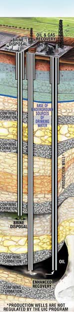
Class 2 UI Wells
Water scarcity from unconventional drilling is a serious concern. According to Ceres analysis, horizontal gas production is far more water intensive than vertical drilling. Also, the liquids that return to the surface from unconventional drilling are often disposed of through deep well injection, which takes the water out of the water cycle permanently. By contrast, water uses are also high for other industries, such as agriculture and electrical generation. However, most of the water used in agriculture and for cooling in power plants eventually returns to the hydrological cycle. It makes its way back into local rivers and water sources.
In the timeframe of this study, Ceres reports that:
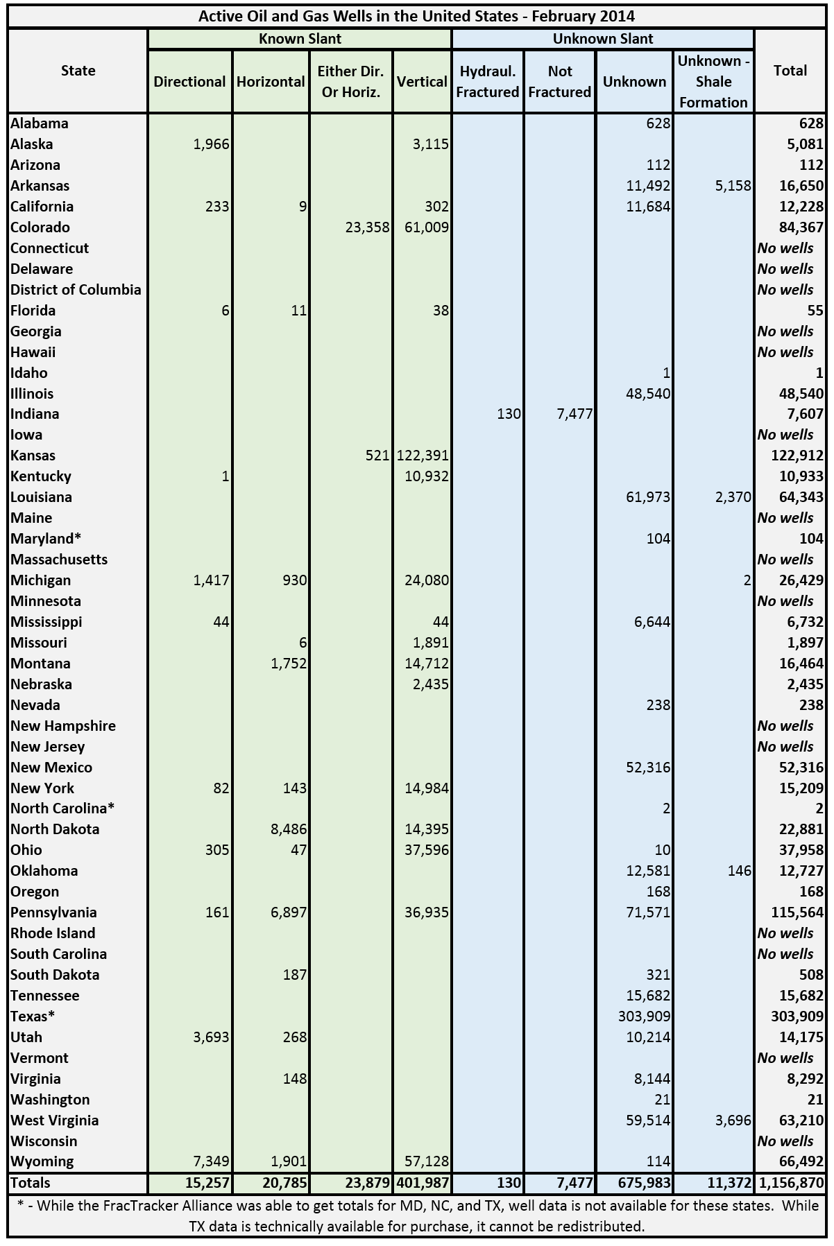
- 97 billion gallons of water were used, nearly half of it in Texas, followed by Pennsylvania, Oklahoma, Arkansas, Colorado and North Dakota, equivalent to the annual water need of 55 cities with populations of ~ 5000 each.
- Over 30 counties used at least one billion gallons of water.
- Nearly half of the wells hydraulically fractured since 2011 were in regions with high or extremely high water stress, and over 55% were in areas experiencing drought.
- Over 36% of the 39,294 hydraulically fractured wells in the study overlay regions experiencing groundwater depletion.
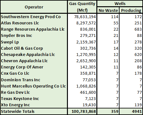
- The largest volume of hydraulic fracturing water, 25 billion gallons, was handled by service provider, Halliburton.
Water withdrawals required for hydraulic fracturing activities have several worrisome impacts. For high stress and drought-impacted regions, these withdrawals now compete with demands for drinking water supplies, as well as other industrial and agricultural needs in many communities. Often this demand falls upon already depleted and fragile aquifers and groundwater. Groundwater withdrawals can cause land subsidence and also reduce surface water supplies. (USGS considers ground and surface waters essentially a single source due to their interconnections). In some areas, rain and snowfall can recharge groundwater supplies in decades, but in other areas this could take centuries or longer. In other areas, aquifers are confined and considered nonrenewable. (We will look at these and additional impact in more detail in our next installments.)
Challenges of documenting water consumption and scarcity
Tracking water volumes and locations turns out to be a particularly difficult process. A combination of factors confuse the numbers, like conflicting data sets or no data, state records with varying criteria, definitions and categorization for waste, unclear or no records for water volumes used in refracturing wells or for well and pipeline maintenance.
Along with these impediments, “chain of custody” also presents its own obstacles for attempts at water bookkeeping. Unconventional drilling operations, from water sourcing to disposal, are often shared by many companies on many levels. There are the operators making exploration and production decisions who are ultimately liable for environmental impacts of production. There are the service providers, like Halliburton mentioned above, who oversee field operations and supply chains. (Currently, service providers are not required to report to FracFocus.) Then, these providers subcontract to specialists such as sand mining operations. For a full cradle-to-grave assessment of water consumption, you would face a tangle of custody try tracking water consumption through that.
To further complicate the tracking of this industry’s water, FracFocus itself has several limitations. It was launched in April 2011 as a voluntary chemical disclosure registry for companies developing unconventional oil and gas wells. Two years later, eleven states direct or allow well operators and service companies to report their chemical use to this online registry. Although it is primarily intended for chemical disclosure, many studies, like several of those cited in this article, use its database to also track water volumes, simply because it is one of the few centralized sources of drilling water information. A 2013 Harvard Law School study found serious limitations with FracFocus, citing incomplete and inaccurate disclosures, along with a truly cumbersome search format. The study states, “the registry does not allow searching across forms – readers are limited to opening one PDF at a time. This prevents site managers, states, and the public from catching many mistakes or failures to report. More broadly, the limited search function sharply limits the utility of having a centralized data cache.”
To further complicate water accounting, state regulations on water withdrawal permits vary widely. The 2011 study by Resources for the Future uses data from the Energy Information Agency to map permit categories. Out of 30 states surveyed, 25 required some form of permit, but only half of these require permits for all withdrawals. Regulations also differ in states based on whether the withdrawal is from surface or groundwater. (Groundwater is generally less regulated and thus at increased risk of depletion or contamination.) Some states like Kentucky exempt the oil and gas industry from requiring withdrawal permits for both surface and groundwater sources.
Can we treat and recycle oil and gas wastewater to provide potable water?
 Will recycling unconventional drilling wastewater be the solution to fresh water withdrawal impacts? Currently, it is not the goal of the industry to recycle the wastewater to potable standards, but rather to treat it for future hydraulic fracturing purposes. If the fluid immediately flowing back from the fractured well (flowback) or rising back to the surface over time (produced water) meets a certain quantity and quality criteria, it can be recycled and reused in future operations. Recycled wastewater can also be used for certain industrial and agricultural purposes if treated properly and authorized by regulators. However, if the wastewater is too contaminated (with salts, metals, radioactive materials, etc.), the amount of energy required to treat it, even for future fracturing purposes, can be too costly both in finances and in additional resources consumed.
It is difficult to find any peer reviewed case studies on using recycled wastewater for public drinking purposes, but perhaps an effective technology that is not cost prohibitive for impacted communities is in the works. In an article in the Dallas Business Journal, Brent Halldorson, a Roanoke-based Water Management Company COO, was asked if the treated wastewater was safe to drink. He answered, “We don’t recommend drinking it. Pure distilled water is actually, if you drink it, it’s not good for you because it will actually absorb minerals out of your body.”
Can we use sources other than freshwater?
How about using municipal wastewater for hydraulic fracturing? The challenge here is that once the wastewater is used for hydraulic fracturing purposes, we’re back to square one. While return estimates vary widely, some of the injected fluids stay within the formation. The remaining water that returns to the surface then needs expensive treatment and most likely will be disposed in underground injection wells, thus taken out of the water cycle for community needs, whereas municipal wastewater would normally be treated and returned to rivers and streams.
Could brackish groundwater be the answer? The United States Geological Survey defines brackish groundwater as water that “has a greater dissolved-solids content than occurs in freshwater, but not as much as seawater (35,000 milligrams per liter*).” In some areas, this may be highly preferable to fresh water withdrawals. However, in high stress water regions, these brackish water reserves are now more likely to be used for drinking water after treatment. The National Research Council predicts these brackish sources could supplement or replace uses of freshwater. Also, remember the interconnectedness of ground to surface water, this is also true in some regions for aquifers. Therefore, pumping a brackish aquifer can put freshwater aquifers at risk in some geologies.
Contaminated coal mine water – maybe that’s the ticket? Why not treat and use water from coal mines? A study out of Duke University demonstrated in a lab setting that coal mine water may be useful in removing salts like barium and radioactive radium from wastewater produced by hydraulic fracturing. However, there are still a couple of impediments to its use. Mine water quality and constituents vary and may be too contaminated and acidic, rendering it still too expensive to treat for fracturing needs. Also, liability issues may bring financial risks to anyone handling the mine water. In Pennsylvania, it’s called the “perpetual treatment liability” and it’s been imposed multiple times by DEP under the Clean Streams Law. Drillers worry that this law sets them up somewhere down the road, so that courts could hold them liable for cleaning up a particular stream contaminated by acid mine water that they did not pollute.
More to come on hydraulic fracturing and water scarcity
Although this article touches upon some of the issues presented by unconventional drilling’s demands on water sources, most water impacts are understood and experienced most intensely on the local and regional level. The next installments will look at water use and loss in specific states, regions and watersheds and shine a light on areas already experiencing significant water demands from hydraulic fracturing. In addition, we will look at some of the recommendations and solutions focused on protecting our precious water resources.

