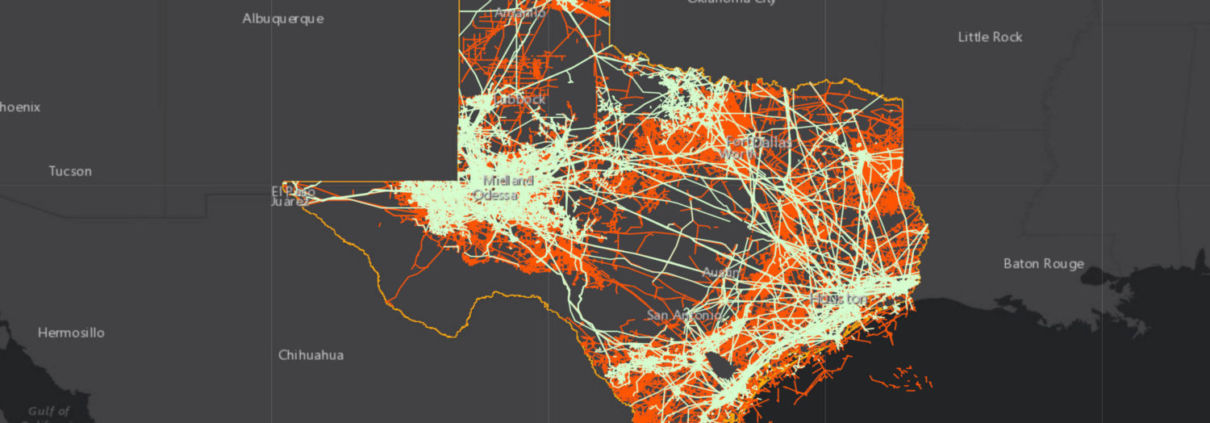
Infrastructure Networks in Texas
This map illustrates infrastructure networks in Texas and explores how these unseen webs connect us and improve lives, but also carry risks and burdens.
This map illustrates infrastructure networks in Texas and explores how these unseen webs connect us and improve lives, but also carry risks and burdens.
We first released this map in February of 2020. In the year since, the world’s energy systems have experienced record changes. Explore the interactive map, updated by FracTracker Alliance in April, 2021.
FracTracker’s aerial survey of unconventional oil & gas infrastructure and activities in northeast PA to southern OH and central WV
Air pollution from Pennsylvania shale gas compressor stations is a significant, worsening public health concern.
By Cynthia Walter, Ph.D.
Dr. Walter is a retired biology professor who has worked on shale gas industry pollution since 2009 through Westmoreland Marcellus Citizens Group, Protect PT and other groups. Contact: walter.atherton@gmail.com
Compressor Stations (CS) in the gas industry are sources of serious air pollutants known to harm humans and the environment. CS are permanent facilities required to transport gases from wells to major pipelines and along pipelines. Additional operations and equipment located at CS also emit toxins. In the last 20 years, CS abundance and sizes have dramatically increased in shale gas extraction areas across the US. This report will focus on CS in and near Southwestern Pennsylvania. Numbers of CS there have risen more than tenfold in the last decade in response to well completions and pipelines after the local fracking boom began in 2005. For example, Westmoreland County, Pennsylvania, had two CS before 2005 and now has 50 CS corresponding with about 341 active shale gas wells. In Pennsylvania, state regulations allow CS to be as close as 750 feet from homes, schools, and businesses. Emission monitoring relevant to public health exposure is limited or absent.
Current Pennsylvania policies allow rapid CS expansion. Also, regulations do not address public health risks due to several major flaws. First, permits allow annual totals of emitted toxins using models that assume constant releases, but substantial emissions from CS occur in peaks that expose citizens to concentrations may impair health, ranging from asthma to cancer. Second, permits do not address the fact that CS simultaneously release many serious air toxins including benzene and formaldehyde, and particulates that carry toxins into lungs. This allowance of multiple toxin release does not reflect the well-established science that public health risks multiply when people are exposed to several toxins at once. Third, permit reviews rarely consider nearby known air pollution sources contributing to aggregate air toxin exposures that occur in bursts and continually. Fourth, permits do not require operators to provide public access to real-time reports of air pollutants released by CS and ambient air quality near CS.
Poor air quality causes harm directly, e.g. respiratory distress, and indirectly, e.g., through increased vulnerability to respiratory viruses. The annual cost of damages from air pollution from CS was estimated at $4 million-$24 million in Pennsylvania based on emissions from CS in 2011. These damages include harm to human and livestock health and losses of crops and timber. After 2011, CS and gas infrastructures continue to expand, with increasing air pollution and damages, especially in shale gas areas. These costs must be compared to the benefits of using alternative energy sources. For example, in a neighboring state, New York, shifting to renewable energy will save tens of billions of dollars annually in air pollution costs, prevent thousands of premature deaths each year, and trigger substantial job creation, based on peer-reviewed research using US government data.
Chemistry of Compressor Station Emissions
Health Effects of Compressor Station Emissions
Regional Air Toxins and Cancer Risk in Southwestern Pennsylvania
Measurements of Compressor Station Emissions
Costs of Compressor Stations and Air Pollution
Appendix – Compressor Station Locations in Westmoreland County, Pennsylvania
CS emissions contribute major air pollutants to the total pollution from unconventional gas development (UCGD), but their role in regional air quality problems has not always been noted. In 2009, when UCGD operations were only a few years in this region and many CS had not yet been built, CS emissions were estimated to be a small component. Now, in 2020, gas transport requirements have increased, leading to many more and larger CS. The amounts of CS emissions have increased accordingly, based on estimates by Carnegie Mellon University atmospheric researcher, Robinson (Figure 1). Part of the reason that CS are such a major pollution source is that they run constantly, in contrast to machinery for well development and trucking that fluctuate with the market for new wells.
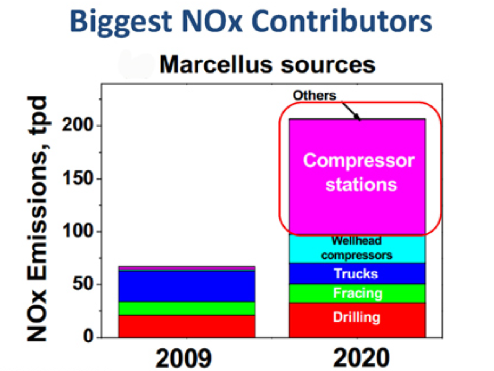
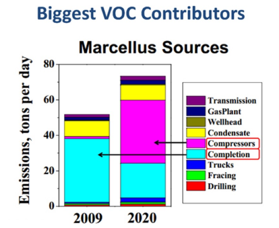
Figure 1. Relative contribution of compressor stations and other components of shale gas industry to Nitrous Oxides (NOx) and Volatile Organic Compounds (VOC). Source: Clean Air Council- adapted from webinar by Alan Robinson.
Air pollutants in CS emissions vary substantially in chemistry and concentrations due to differences in equipment (Table 1). Emissions in CS can come from several types of sources described below.
“In the Fort Worth, TX area, researchers evaluated compressor station emissions from eight sites, focusing in part on fugitive emissions. A total of 2,126 fugitive emission points were identified in the four month field study of 8 compressor stations: 192 of the emission points were valves; 644 were connectors (including flanges, threaded unions, tees, plugs, caps and open-ended lines where the plug or cap was missing); and 1,290 were classified as Other Equipment. The Other category consists of all remaining components such as tank thief hatches, pneumatic valve controllers, instrumentation, regulators, gauges, and vents. 1,330 emission points were detected with an IR camera (i.e. high-level emissions) and 796 emission points were detected by Method 21 screening (i.e. low-level emissions). Pneumatic Valve Controllers were the most frequent emission sources encountered at well pads and compressor stations.”
Eastern Research Group (2011).
Table 1. Examples of air pollutants allowed for release by compressor stations. Air pollutants (pounds/year) are estimates provided by the companies for permits in West Virginia and Pennsylvania in recent years. Total compressor engine horsepower (hp) is noted. Sources: Janus and Tonkin CS Permits at WV DEP website. Shamrock CS permit. Buffalo CS, Washington, Co PA – PENNSYLVANIA BULLETIN, VOL. 45, NO. 16 APRIL 18, 2015.
| Pollutant | Term | Janus (WV)
22,000 hp |
Tonkin (WV)
4390 hp |
Shamrock* (PA)
4140 bhp |
Buffalo ** (PA) 20,000 hp + 5,000 bhp |
| Nitrogen Oxides | NOx | 254,400 | 248,000 | 170,000 | 155,800 |
| Volatile Organic Compounds | VOC | 191,200 | 30,000 | 66,000 | 77,000 |
| Carbon Monoxide | CO | 118,200 | 80,000 | 154,000 | 144,400 |
| Sulfur Dioxide | SO2 | 1,400 | 400 | 10,000 | 5,400 |
| Hazardous Air Pollutants-Total | HAP | 48,200 | 3,280 | 19,400 | 30,000 |
| Formaldehyde | 1,080 | 12,800 | 12,200 | ||
| Benzene | 540 | ||||
| Ethylbenzene | 60 | ||||
| Toluene | 140 | ||||
| Xylene | 200 | ||||
| Hexane | 500 | ||||
| Acetaldehyde | 600 | ||||
| Acrolein | 160 | ||||
| Total Particulate Matter
(PM-2.5, PM-10-separate or combined) |
PM | 18,200 | 11,000 | 32,000 | PM-10 32,000
PM-2.5 32,000 |
| TOTAL TOXINS | 631,600 | 372,680 | 417,400 | 444,600 | |
| Carbon Dioxide Equivalents | CO2-e | 29,298,000 | 27,200,000 | 367,000,000 | 214,514,000 |
Several toxic chemicals are released by individual CS in amounts that range from a few thousand pounds to a quarter of a million pounds per year (Tables 1 & 2) as described below.
Health impacts from many of the substances released by CS are well-known in medical research. For example, many of the VOC and HAP compounds permitted for release by state agencies are known carcinogens (Table 3). Many of these substances also impact the nervous system as shown in the organic compounds measured in CS in PA and listed in Table 4. Also, a study of 18 CS in New York by Russo and Carpenter (2017) found that all 18 CS released substances with known impacts on the nervous system and total annual emissions were over five million pounds, among the highest of all types of emissions (Table 5). Russo and Carpenter also found high annual emissions of over five million pounds for substances known to be associated with each of the following other health problems: digestive problems, circulatory disorders, and congenital malformations.
Congenital defects were significantly more common for mothers living in a 10-mile radius of denser shale gas development in Colorado compared to reference populations (MacKenzie et al. 2014). Currie et al. (2017) examined over a million birth records in Pennsylvania and found statistically significant increased frequencies of low birth weight and negative health scores for infants born to mothers within 3 km of unconventional gas wells compared to matching populations more distant from shale gas developments. Such developments include a wide range of gas infrastructure including CS and also high truck traffic and fracking. One plausible mechanism for harm to developing babies is exposure to VOCs such as benzene, toluene and xylene associated with CS and well operations. These VOC’s are classified by the Agency for Toxic Substances and Disease Registry as known to cross the placental barrier and cause harm to the fetus including birth deformities.
In sum, CS are a significant source of air pollutants with direct and indirect impacts on health. One indirect impact especially important during the COVID-19 pandemic in 2020, is the increased incidence and severity of respiratory viral infections in populations living in areas with poor air quality. Ciencewicki, and Jaspers (2007) write, “a number of studies indicate associations between exposure to air pollutants and increased risk for respiratory virus infections.”
Table. 2. Health effects of air pollutants permitted for release by compressor stations.
| Pollutant | Health Effects |
| Particulate Matter | Impairs lungs and transfers toxins into body when microscopic particles carry chemicals deep into lungs and release into bloodstream. |
| Nitrogen Oxides |
Forms ozone that impairs lung function which can trigger asthma and heart attacks and scars lungs in the long term. Forms acid rain that dissolves toxic metals into water supplies. |
| Volatile Organic Compounds | Includes a wide variety of gaseous organic compounds, some of which cause cancer. Many VOC react to form ozone that impairs lungs as noted above. |
| Carbon Monoxide | Blocks ability of blood to carry oxygen.
Also forms ozone that impairs lungs as noted above. |
| Sulfur Dioxide | Irritates lungs, triggering respiratory and heart distress.
Forms acid rain that dissolves toxic metals into water supplies. |
| Hazardous Air Pollutants | Category of various toxic compounds many of which impact the nervous system. Includes formaldehyde, benzene and several other carcinogens. |
| Total Toxins | Sum of emissions of all toxins. Exposure to multiple toxins exacerbates harm directly through impairment of lungs and circulatory system and indirectly through injury to detoxification mechanisms, such as liver function. |
| Carbon Dioxide Equivalents | A measure of the combined effects of greenhouse gases such as CO2 and Methane expressed in a standard unit equivalent to the heat trapping effect of CO2. Greenhouse gases trap heat and worsen climate change and related harm to health when increased air temperatures directly cause stress directly and indirectly accelerate ozone formation. |
Table 3. Gas industry list of carcinogenicity rating for Hazardous Air Pollutants (HAPs) released by compressor stations in a factsheet prepared by EQT for Janus compressor, WV. 2015 Source: DEP.
| Substance | Type | Known/Suspected Carcinogen | Classification |
| Acetaldehyde | VOC | Yes | B2-Probable Human Carcinogen |
| Acrolein | VOC | No | Inadequate Data |
| Benzene | VOC | Yes | Category A – Known Human Carcinogen |
| Ethyl-benzene | VOC | No | Category D Not Classifiable |
| Biphenyl | VOC | Yes | Suggested Evidence of Carcinogenic Potential |
| 1,3 Butadiene | VOC | Yes | B2-Probable Human Carcinogen |
| Formaldehyde | VOC | Yes | B1- Probable Human Carcinogen |
| n-Hexane | VOC | No | Inadequate Data |
| Naphthalene | VOC | Yes | C- Possible human Carcinogen |
| Toluene | VOC | No | Inadequate Data |
| 2,3,4-Trimethlypentane | VOC | No | Inadequate Data |
| Xylenes | VOC | No | Inadequate Data |
Table 4. Center for Disease Control list of health effects for volatile organic carbons measured by PA DEP near compressor station. Source: CDC.
| Substance | Exposure Symptoms | Target Organs |
| Ethylbenzene | Irritation to eyes and nose; nausea, headache; neuropath; numb extremities, muscle weakness; dermatitis; dizziness | Eyes, skin, respiratory system, central nervous system, peripheral nervous system |
| n-Butane | Drowsiness | Central nervous system |
| n-Hexane | Irritation to eyes, skin & respiratory system; headache, dizziness; nausea | Eyes, skin, respiratory system, central nervous system |
| 2-Methyl Butane | n/a | n/a |
| Iso-butane | Drowsiness, narcosis, asphyxia | Central nervous system |
Table 5. Amounts of pollutants known to be associated with health impacts in a review of 18 New York compressor stations. Emissions were grouped and tallied based on their impacts on disorders classified by ICD codes as defined by the International Statistical Classification of Diseases and Related Health Problems (ICD), a medical classification list by the World Health Organization. Source: Copy of Table 3.17b, Russo and Carpenter 2017.
| ICD-10 | Facilities | Chemicals | Pounds | ||||||||||||
| # | Description | ‘08 | ‘11 | ‘14 | Tot | ‘08 | ‘11 | ‘14 | Tot | 2008 | 2011 | 2014 | Total | ||
| 1 | Q00-Q89 | Congenital malformations and deformations | 18 | 18 | 17 | 18 | 57 | 54 | 54 | 57 | 4,393,806 | 6,607,676 | 5,900,691 | 16,902,175 | |
| 1.1 | Q00-Q07 | Nervous system | 18 | 18 | 17 | 18 | 16 | 16 | 16 | 16 | 4,068,877 | 5,882,704 | 5,258,344 | 15,209,926 | |
| 1.2 | Q10-Q18 | Eye, ear, face and neck | 15 | 15 | 12 | 15 | 4 | 4 | 4 | 4 | 5,825 | 19,569 | 11,475 | 36,869 | |
| 1.3 | Q20-Q28 | Circulatory system | 18 | 18 | 17 | 18 | 10 | 10 | 10 | 10 | 4,269,779 | 6,336,905 | 5,651,896 | 16,258,581 | |
| 1.4 | Q30-Q34 | Respiratory system | 14 | 8 | 7 | 14 | 4 | 4 | 4 | 4 | 150 | 107 | 113 | 372 | |
| 1.5 | Q35-Q45 | Digestive system | 18 | 18 | 17 | 18 | 17 | 17 | 17 | 17 | 4,386,043 | 6,586,345 | 5,884,324 | 16,856,713 | |
| 1.6 | Q50-Q56 | Genital organs | 6 | 7 | 8 | 8 | 2 | 2 | 2 | 2 | 1,399 | 4,373 | 2,612 | 8,385 | |
| 1.7 | Q60-Q64 | Urinary system | 18 | 17 | 16 | 18 | 9 | 9 | 9 | 9 | 119,382 | 254,922 | 237,359 | 611,663 | |
| 1.8 | Q65-Q79 | Musculoskeletal system | 18 | 18 | 16 | 18 | 19 | 19 | 19 | 19 | 122,314 | 262,300 | 243,932 | 628,547 | |
| 1.9 | Q80-Q89 | Other | 18 | 18 | 17 | 18 | 55 | 52 | 52 | 55 | 2,124,445 | 3,614,575 | 3,413,375 | 9,152,395 | |
| 2 | Q90-Q99 | Chromosomal abnormalities, nec | 18 | 18 | 16 | 18 | 30 | 31 | 31 | 32 | 120,669 | 256,739 | 239,709 | 617,118 | |
| Q00-Q99 | Total | 18 | 18 | 17 | 18 | 57 | 56 | 56 | 59 | 4,393,806 | 6,607,676 | 5,900,691 | 16,902,175 | ||
Cancer risks from HAPs have been elevated for many years in several areas of Southwestern PA, as noted in a map from 2005 (Figure 2), when most air pollution was from urban traffic and single sources such as coke works and unconventional gas development (UCGD) had just begun in the region. The cancer risk pattern changed by 2014 (Figure 3). The specific numbers of excess cancer risk predicted for each location cannot be compared between the two maps because each map was produced using different sources of information and models. The pattern, however, can be compared and shows that elevated cancer risk is now more widespread across Southwestern PA and no longer primarily in Allegheny County.
Cancer risk maps are constructed by the EPA office of National Air Toxics Assessment (NATA) using models of reported air toxics and their relationship to cancer as a risk factor, as defined by NATA: “A risk level of “N”-in-1 million implies that up to “N” people out of one million equally exposed people would contract cancer if exposed continuously (24 hours per day) to the specific concentration over 70 years (an assumed lifetime). This would be in addition to cancer cases that would normally occur in one million unexposed people.” (https://www.epa.gov/national-air-toxics-assessment/nata-glossary-terms) In the current context, the NATA models are useful to compare the relative differences in air quality from a public health perspective, assuming the data on air pollutants is complete.
Another, very different statistic regarding cancer is the rate of cancer, also called the incidence. This number is based on actual reported cases and applies to cancers that occur due to all causes. The cancer rate, therefore, is a much higher number than a risk factor. For example, according to the US Center for Disease Control, the annual rate of new cases of cancer in PA in 2016, the most recent year reported, was 482.5 per 100,000 people. Compared to other states, PA is among the ten states with the highest cancer incidence. In the US, one in four people die from cancer, placing it second to heart disease as a leading cause of death. (https://gis.cdc.gov/Cancer/USCS/DataViz.html). Compared to other nations, the US has the fifth highest cancer rate, with 352 new cases each year per 100,000 people. (https://www.wcrf.org/dietandcancer/cancer-trends/data-cancer-frequency-country)
Compressor station emissions contribute to air pollutants known to be associated with cancer. For example, in a review of emissions for 18 CS in New York, Russo and Carpenter (2017) found that most or all CS released substances associated with a wide range of cancers (Table 6). Up to 56 such chemicals were emitted in amounts that totaled over 1 million pounds each year.
Maps of cancer risk are likely to be under-reporting risk levels in both the amount rates of risk and also the locations. Cancer risks from serious air pollutants cannot be properly mapped for several reasons. First, reports on concentrations of HAP in emissions are limited. HAP emissions are in accounts required only from large facilities, and thus, smaller operations, such as many CS, are likely be ignored. Second, general air quality monitoring stations are limited in location and do not measure HAP. For example, the PA DEP maintains 47 air quality stations dispersed among over 60 counties (http://www.dep.state.pa.us/dep/deputate/airwaste/aq/aqm/pollt.html). Most stations report hourly measures of Ozone and PM-2.5, and only a handful also monitor one or more other substances such as CO, NOx, SO ₂ or H2S. One county in Southwestern PA has additional air quality stations. Allegheny has a county health department that maintains 17 stations to report real-time air quality based on Ozone, SO2 or PM-2.5 (https://alleghenycounty.us/Health-Department/Programs/Air-Quality/Air-Quality.aspx).
In sum, cancer risk estimates from air pollution fall short in the following ways:
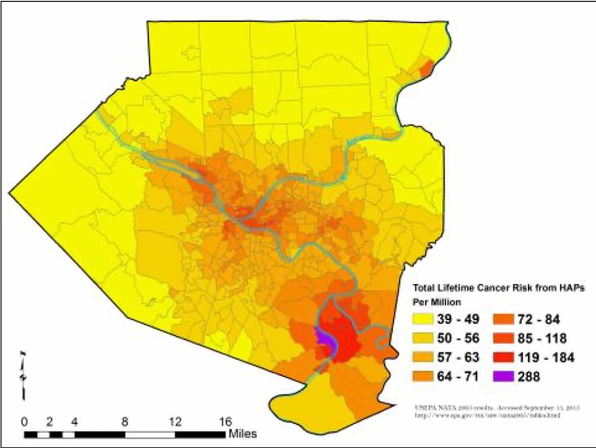
Figure 2. Cancer risk map in Southwestern Pennsylvania in 2005 from the National Air Toxics Assessment program in the EPA. Total Lifetime Cancer Risk from Hazardous Air Pollutants (HAP) per million. Colors indicate yellow for 28-78, gold for 79-95, light orange for 99-148, orange for 149-271, bright orange for 272-517, and red for 518-744 excess cancer risk per million. (https://www.epa.gov/national-air-toxics-assessment)

Figure 3. Cancer risk map in Southwestern Pennsylvania in 2014 from the National Air Toxics Assessment in the EPA. Facilities are locations where air quality information was available for modeling. Total Risk of cancer as a baseline was assumed to be 1 per 1,000,000. Estimates of risk predict known air pollution sources alone will cause 1-24 excess cancers per million in Light Pink areas, 25-49 excess cancers per million in Gray areas, and 50-74 excess cancers per million in Blue areas. Source: EPA.
Table 6. Amounts of pollutants known to be associated with cancer in a review of 18 New York compressor stations. Emissions were grouped and tallied based on their impacts on disorders classified by ICD codes as defined by the International Statistical Classification of Diseases and Related Health Problems (ICD), a medical classification list by the World Health Organization. Source: Copy of Table 3b, Russo and Carpenter 2017.
| ICD-10 | Facilities | Chemicals | Pounds | |||||||||||
| # | Code | Description | ‘08 | ‘11 | ‘14 | Tot | ‘08 | ‘11 | ‘14 | Tot | 2008 | 2011 | 2014 | Total |
| 1 | C00-C97 | Malignant neoplasms | 18 | 18 | 17 | 18 | 53 | 54 | 54 | 56 | 744,394 | 1,679,621 | 1,583,745 | 4,007,761 |
| 2 | C00-C14 | Lip, oral cavity and pharynx | 18 | 18 | 16 | 18 | 12 | 14 | 14 | 14 | 118,992 | 254,897 | 238,943 | 612,833 |
| 3 | C15-C26 | Digestive organs | 18 | 18 | 16 | 18 | 37 | 38 | 38 | 38 | 121,690 | 258,670 | 241,866 | 622,227 |
| 4 | C30-C39 | Respiratory system and intrathoracic organs | 18 | 18 | 17 | 18 | 36 | 37 | 37 | 38 | 740,798 | 1,673,574 | 1,579,882 | 3,994,254 |
| 5 | C40-C41 | Bone and articular cartilage | 18 | 18 | 17 | 18 | 33 | 34 | 34 | 35 | 694,106 | 1,551,399 | 1,492,704 | 3,738,210 |
| 6 | C43-C44 | Skin | 16 | 15 | 13 | 16 | 12 | 12 | 12 | 14 | 2,362 | 5,008 | 4,029 | 11,400 |
| 7 | C45-C49 | Connective and soft tissue | 17 | 17 | 15 | 17 | 17 | 17 | 17 | 17 | 1,929 | 5,074 | 4,639 | 11,643 |
| 8 | C50-C58 | Breast and female genital organs | 18 | 18 | 16 | 18 | 23 | 25 | 25 | 25 | 361,015 | 823,303 | 663,237 | 1,847,556 |
| 9 | C60-C63 | Male genital organs | 18 | 17 | 16 | 18 | 12 | 13 | 13 | 13 | 111,217 | 233,176 | 224,147 | 568,541 |
| 10 | C64-C68 | Urinary organs | 18 | 18 | 16 | 18 | 24 | 24 | 24 | 25 | 119,062 | 255,474 | 238,596 | 613,133 |
| 11 | C69-C72 | Eye, brain and central nervous system | 18 | 18 | 16 | 18 | 20 | 20 | 20 | 20 | 121,282 | 258,655 | 241,954 | 621,892 |
| 12 | C73-C75 | Endocrine glands and related structures | 18 | 17 | 16 | 18 | 10 | 10 | 10 | 10 | 112,911 | 235,120 | 225,269 | 573,300 |
| 13 | C76-C80 | Secondary and ill-defined | 17 | 16 | 14 | 17 | 6 | 6 | 6 | 6 | 2,054 | 5,690 | 5,771 | 13,516 |
| 14 | C81-C96 | Malignant neoplasms, stated or presumed to be primary, of lymphoid, haematopoietic and related tissue | 18 | 18 | 16 | 18 | 31 | 31 | 31 | 31 | 364,338 | 833,140 | 671,245 | 1,868,724 |
| 15 | C97 | Malignant neoplasms of independent (primary) multiple sites | 0 | 0 | 0 | 0 | 0 | 0 | 0 | 0 | 0 | 0 | 0 | 0 |
| 16 | D00-D09 | In situ neoplasms | 16 | 15 | 13 | 16 | 3 | 3 | 3 | 3 | 3,313 | 7,557 | 6,606 | 17,477 |
| 17 | D10-D36 | Benign neoplasms | 17 | 17 | 14 | 17 | 27 | 27 | 27 | 27 | 12,499 | 35,013 | 23,068 | 70,580 |
| 18 | D37-D48 | Neoplasms of uncertain or unknown behavior | 18 | 18 | 16 | 18 | 39 | 40 | 40 | 41 | 121,277 | 257,142 | 240,115 | 618,535 |
Studies of real-world concentrations of air pollutants from CS emissions are lacking, but some reports exist. Of these, a few records are in peer-reviewed studies, and cited in reviews such as Saunders et al. 2018. A few published reports are described below. They all show the high variation over time for CS emissions and the occurrence of peak concentrations.
Macey et al. (2014) observed ambient air near CS contained toxins at concentrations that impair health. They collected grab samples of air from industrial sites including CS in Arkansas and Pennsylvania and analyzed them for toxins using EPA approved methods. Most of the CS studied in Arkansas (Table 6) and Pennsylvania (Table 7) released formaldehyde at amounts associated with a cancer risk from exposure to this substance of 1/10,000 which is equivalent to 100 times higher risk than the widely accepted baseline risk of 1 per million. This means the amounts of formaldehyde found near CS substantially increased the risk of cancer using well-established federal analyses (https://www.atsdr.cdc.gov/hac/phamanual/appf.html). Some toxins Macey et al. recorded are less well studied than formaldehyde and benzene. For example, 1,3-butadiene is classified by the EPA as a known human carcinogen, but a calculation of cancer risk for this substance is lacking. Air samples in the Macey study were collected close to the CS (e.g., 30-42m) and at greater distances (e.g., 254-460m). Those distant samples were well beyond the 750-foot set-back rule for Pennsylvania. At all these distances, air movement modeling predicts that toxins released from a source such as a CS are likely to travel downwind within the air mass under most weather conditions, thus exposing residents near and further from CS. Many people, therefore, in homes, schools and businesses that are downwind of CS are likely to experience serious air toxins at concentrations that harm their health.
Air toxins were also measured by the Pennsylvania Department of Environmental Protection in 2010 in a variety of unconventional gas extraction facilities including one CS in Washington County, PA. Brown et al. (2015) reported these data, showing the concentrations that citizens could experience near a compressor station varied greater than tenfold within a day and among consecutive days (Table 8). The length of time for peak concentrations was unknown, but Brown et al. used a model of weather including wind patterns to estimate citizens are likely to experience 118 peak concentrations per year.
Goetz et al. (2015) sampled air in Marcellus shale regions of Pennsylvania for short periods (1-2.5 hrs.) at distances 480-1100 meters from eight CS, four with relatively small capacity (5,000-9,000 hp) and four with moderate capacity (14,000-17,000 hp). They found that each CS had a different pattern of relatively higher concentrations of some pollutants, such as NOX versus other pollutants, e.g., CO. Also, totals of all pollutants did not correlate with compressor engine capacity, probably because the CS they sampled include a mix of engines using fossil fuels and electric power. Goetz et al. concluded with recommendations for more comprehensive and longer-term monitoring to better understand air pollution from CS and all components in shale gas development.
Radionuclides in CS emissions are almost never measured, even though Marcellus shales are well known for containing elevated amounts of radiologic substances such as uranium, radium and radon. The only published report of testing for radionucleotides in CS emissions in PA was a test of a single CS emission for one period of time. In a review of radiation in shale gas industry components, the Pennsylvania Department of Environmental Protection (PA DEP) measured radon (Rn) in ambient air at one CS by deploying sample bags in four cardinal directions at the fence line at a height of 5 feet for 62 days. They reported Rn concentrations of 0.1-0.8 pCi/L, values they stated were within the range of outdoor air in the US. (https://www.dep.pa.gov/Business/Energy/OilandGasPrograms/OilandGasMgmt/Oil-and-Gas-Related-Topics/Pages/Radiation-Protection.aspx) Given the high variation of amounts of emissions from CS and variable chemistry in sources of gases released from combustion, blowdowns and leaks, frequent testing for radionucleotides should be standard in monitoring CS emissions.
Methane is the substance tracked most often in emissions from CS and other gas industry facilities because of its central role in operations, requirements to avoid explosive concentrations, and readily available measurement technology, in comparison to other substances emitted from CS. Although methane emissions from CS are not always correlated with amounts of other, more toxic emissions, patterns observed in plumes of methane from CS are likely to reflect elevated concentrations of other harmful substances from CS.
Nathan et al (2015) sampled methane emissions from one CS in the Barnett shale region using a sensor carried on a model aircraft. The open-path, laser sensor produced measures with a precision of 0.1 ppmv over short intervals, allowing researchers to see emission variation in time and space as the aircraft changed position. Based on 22 flights within a week period, they observed a substantial range in methane released from 0.3 – 73 g CH4 per second. These values calculate to 0.02 – 6.3 metric tons of methane per day, a range that matches that estimated by Goetz of 0.5 – 9 metric tons per day. In addition, Nathan et al. found high variability in concentrations at different heights, as the emission plumes shifted in response to wind velocity, direction and topography. They recommend caution in interpretations of ground-based emission monitors and called for more monitoring of air movements and emissions at different elevations.
Payne et al. 2017 confirmed these ideas when they mapped plumes of methane in CS in New York and Pennsylvania using a sensor capable of recording methane in parts per million (ppm) every 0.25 – 5 seconds. The sensor was located on a mobile unit that marked GPS location. They found high variability in the shape and extent of plumes. For example, one of most extensive plumes was recorded near Dimock, Pennsylvania in a locale with CS as the only major source of methane. Researchers recorded the highest concentrations of methane in the study, 22 ppm, at 500 m from the CS, with a second peak of 0.6 ppm noted over 1 km from the CS and elevated methane as far as 3 km from the site (Figure 4). Wind direction did not always predict the shape of the plume, but data collection was restricted by the path of the sensor and the transport vehicle (Figure 8). Most importantly, they found that …“during atmospheric temperature inversions, when near-ground mixing of the atmosphere is limited or does not occur, residents and properties located within 1 mile of a compressor station can be exposed to rogue methane from these point sources.” These residents are likely to also experience excess toxins from CS as well, especially under such weather conditions.
Exposure to peak concentrations of air pollutants have dramatic effects on health for several reasons. First, lungs carry toxins into the blood within seconds, and the blood quickly transfers compounds to the brain and other vital organs. Many of the substances released by compressor stations impact the central nervous system as seen in Table 3, and these toxins are released simultaneously. Citizens, therefore inhaling a plume of emissions will have impacts from the total of these compounds. The health impacts for these combined toxins are unknown, and especially of concern during pregnancy and child development. Exposure studies in animals and humans test individual substances and the Center for Disease Control and NIOSH use these to develop exposure guidelines for a healthy adult in a work-place. In contrast, residents near compressor stations will include citizens of all ages with various health conditions. For example, the American Lung Association determined that over 50% of the 360,000 residents of Westmoreland County are at greater risk for health impairment due to air pollution because they have one or more of these conditions: asthma, diabetes, heart disease, respiratory illness, advanced age (https://www.lung.org/our-initiatives/healthy-air/sota/key-findings/people-at-risk.html).
In sum, the research on CS emissions of methane, air pollutants such as NOx, and hazardous air pollutants such as formaldehyde and benzene, all indicate exposures to CS emissions pose a threat to public health, but the emissions have not yet been fully quantified and modeled. Documenting CS contributions to harmful ambient air quality is feasible, however. The published studies from as far back as 2011 indicate that instrumentation to record substances and weather are readily available. Activities within a station such as compressor function, blowdowns, venting and flaring are all recorded by operators, but such reports are not released to researchers or the public. The science of models that predict public health risks in response to air pollution exposure are highly developed. In sum, operators of CS have the technology to measure emissions and ambient air quality and scientists have the models, but lack of industry data prevents the public from knowing impacts from CS.
Table 6. Air toxins found in grab samples near Arkansas compressor stations including concentrations, the Agency for Toxic Substances and Disease Registry (ASTDR), Minimum Risk Level (MRL) exceedance, and the Environmental Protection Agency (EPA) Integrated Risk Information System (IRIS) cancer risk. Source: Copy of Table 4 from Macey et al. 2014.
| State/ID | County | Nearest infrastructure | Chemical | Concentration (μg/m3) | ATSDR MRLs
exceeded |
EPA IRIS cancer risk exceeded |
| AR-3136-003 | Faulkner | 355 m from compressor | Formaldehyde | 36 | C | 1/10,000 |
| AR-3136-001 | Cleburne | 42 m from compressor | Formaldehyde | 34 | C | 1/10,000 |
| AR-3561 | Cleburne | 30 m from compressor | Formaldehyde | 27 | C | 1/10,000 |
| AR-3562 | Faulkner | 355 m from compressor | Formaldehyde | 28 | C | 1/10,000 |
| AR-4331 | Faulkner | 42 m from compressor | Formaldehyde | 23 | C | 1/10,000 |
| AR-4333 | Faulkner | 237 m from compressor | Formaldehyde | 44 | C, I | 1/10,000 |
| AR-4724 | Van Buren | 42 m from compressor | 1,3-butadiene | 8.5 | n/a | 1/10,000 |
| AR-4924 | Faulkner | 254 m from compressor | Formaldehyde | 48 | C, I | 1/10,000 |
C = chronic; I = intermediate.
Table 7. Air toxins found in grab samples near Pennsylvania compressor stations including concentrations, the Agency for Toxic Substances and Disease Registry (ASTDR), Minimum Risk Level (MRL) exceedance, and the Environmental Protection Agency (EPA) Integrated Risk Information System (IRIS) cancer risk. Source: Copy of Table 5 from Macey et al. 2014
| State
ID |
County | Nearest infrastructure | Chemical | Concentration (μg/m3) | ATSDR MRLs
exceeded |
EPA IRIS cancer risk exceeded |
| PA-4083-003 | Susquehanna | 420 m from compressor | Formaldehyde | 8.3 | 1/10,000 | |
| PA-4083-004 | Susquehanna | 370 m from compressor | Formaldehyde | 7.6 | 1/100,000 | |
| PA-4136 | Washington | 270 m from PIG launcha | Benzene | 5.7 | 1/100,000 | |
| PA-4259-002 | Susquehanna | 790 m from compressor | Formaldehyde | 61 | C, I, A | 1/10,000 |
| PA-4259-003 | Susquehanna | 420 m from compressor | Formaldehyde | 59 | C, I, A | 1/10,000 |
| PA-4259-004 | Susquehanna | 230 m from compressor | Formaldehyde | 32 | C | 1/10,000 |
| PA-4259-005 | Susquehanna | 460 m from compressor | Formaldehyde | 34 | C | 1/10,000 |
C = chronic; A = acute; I = intermediate.
aLaunching station for pipeline cleaning or inspection tool.
Table 8. Variation in air pollutants measured in ug/cubic meter by PA DEP during two sampling times per day for three consecutive days near a compressor station in Southwest PA. Source: Copied from Table 1. Brown et al. 2015 based on data from Southwestern Pennsylvania Short Term Marcellus Ambient Air Sampling Report, Pennsylvania Department of Environmental Protection, Nov. 2010.
| May 18 | May 19 | May 20 | |||||||
| Chemical | Morning | Evening | Morning | Evening | Morning | Evening | 3-day Average | ||
| Ethylbenzene | No detect | No detect | 964 | 2015 | 10,553 | 27,088 | 13,540 | ||
| n-Butane | 385 | 490 | 326 | 696 | 12,925 | 915 | 5,246 | ||
| n-Hexane | No detect | 536 | 832 | 11,502 | 33,607 | No detect | 15,492 | ||
| 2-Methyl Butane | No detect | 230 | 251 | 5137 | 14,271 | No detect | 6,630 | ||
| Iso-butane | 397 | 90 | No detect | 1481 | 3,817 | 425 | 2070 | ||
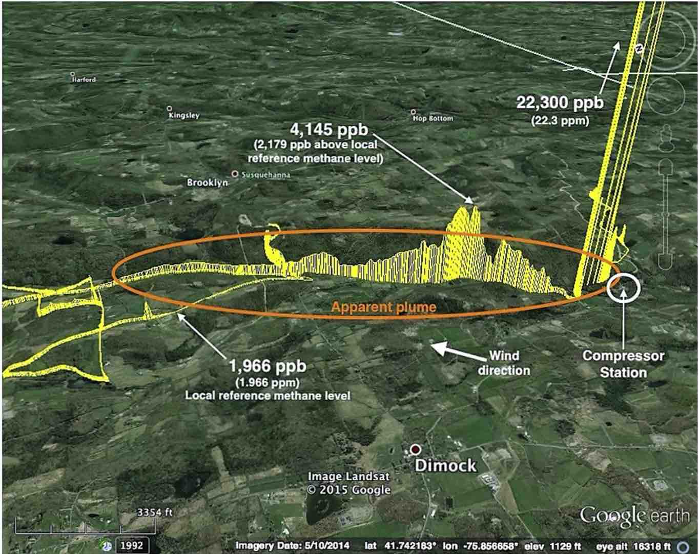
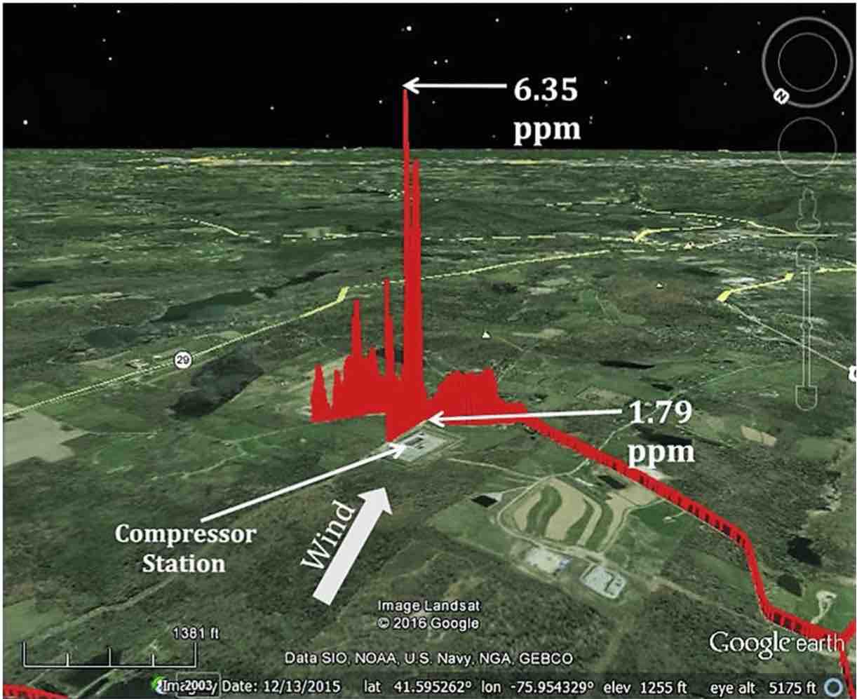
Figure 4. Methane emission plumes from compressor stations near Dimock, Pennsylvania (left) and Springvale, Pennsylvania (right). Source: Copied from Payne et al. 2017.
Prior to 2008, compressor stations were infrequent with one or a few per county broadly distributed across PA as part of gas transport from locations outside of PA (Figure 5). These pipelines were mainly an issue for public health in the case of explosions. Major transmission pipelines use pressures up to 1500 psi. Leaks, therefore, release large amounts of gas much of which is not noticed because it lacks the mercaptan odorant added to household methane. For example, the 30-inch Spectra gas pipeline that exploded in 2016 in Westmoreland County caused a hole 12 feet deep and1500 square feet in area and burned 40 acres. The PA DEP claimed to have measured air quality, but they did not arrive until long after the plume from the fire traveled downwind. This pipeline was transporting gas from one of the largest gas storage facilities in the country, the Sunoco Gas Depot in Delmont, Pennsylvania to New Jersey as part of over 9,000 miles of pipelines in the Texas Eastern system from the Gulf Coast to the Northeast. That section of pipeline was built in 1981 and had recently been increased in pressure, probably using older or newer compressors in nearby locations. Faulty joints between pipeline sections were blamed for the catastrophic release of gas. (Phillips, S. 2016. State Impact, NPR). Immediately after the explosion, while gas continued to pour out of the pipeline, emergency workers needed at least one hour to locate shut-off locations. In general, pipeline shut-offs are sited at compressors stations or at intervals along a pipeline.
CS abundance in counties with shale gas extraction increased over tenfold in the decade after 2005 when the gas industry obtained exemptions to the Clean Water Act and began unconventional gas extraction in Pennsylvania (Figure 6). Permit applications for new wells, pipelines and CS continue throughout southwest Pennsylvania. In PA, the Oil and Gas law states the following: “ In order to allow for the reasonable development of oil and gas resources, a local ordinance … Shall authorize natural gas compressor stations as a permitted use in agricultural and industrial zoning districts and as a conditional use in all other zoning districts, if the natural gas compressor building meets the following standards:….(i) is located 750 feet or more from the nearest existing building or 200 feet from the nearest lot line, whichever is greater, unless waived by the owner of the building or adjoining lot;” (Pennsylvania Statutes Title 58 Pa.C.S.A. Oil and Gas §3304). CS and many aspects of the shale gas industry are controlled by this state law.
Each stage of gas extraction involves emissions that can be close or far from the well pad. Most emissions involve diesel engines. Diesel engines are well-known to produce substantial amounts of VOC’s, NOx and particulate pollution (PM-2.5, PM-10). Well pad construction requires intense activity by diesel trucks and earth moving equipment. Well drilling uses diesel engines. From 3 – 5 million gallons of water are used for each fracking event and up to 300 truck visits are needed to transport water for the many wells that are not close to water supplies from piped sources. Trucks are used to transport the 1 – 2 million gallons of produced water that emerges from the well for disposal in injection wells likely to be distant from most wells. Additional waste is carried long distances as well, including drill cuttings and sludge. For example, shale gas industry waste was handled for years in Max Environmental, one of the largest industrial waste sites in the eastern US located in Yukon, Westmoreland County since the 1960’s. Within one mile of Yukon is Reserved Environmental, a waste facility with operations focused since 2008 on processing sludge from fracking into solid cakes to be trucked to other landfills. In sum, all stages of shale gas industry contribute to many poorly documented sources of air pollution likely to be near CS.
The density of CS in some areas such as southwest Pennsylvania impacts the local and regional air quality. For example, Westmoreland County has 50 CS and 341 shale gas wells (https://www.fractracker.org) and some neighboring counties have even more shale gas emission sources. People in Westmoreland County receive pollutants from shale gas activities in their immediate vicinity and additional air pollutants from CS and other industries in neighboring counties. Wind patterns shown in Figure 7 indicate Westmoreland County is frequently downwind from Washington County, a county with a very high density of shale gas operations, and Eastern Allegheny County where large industries such as coke works release substantial amounts of air pollutants.
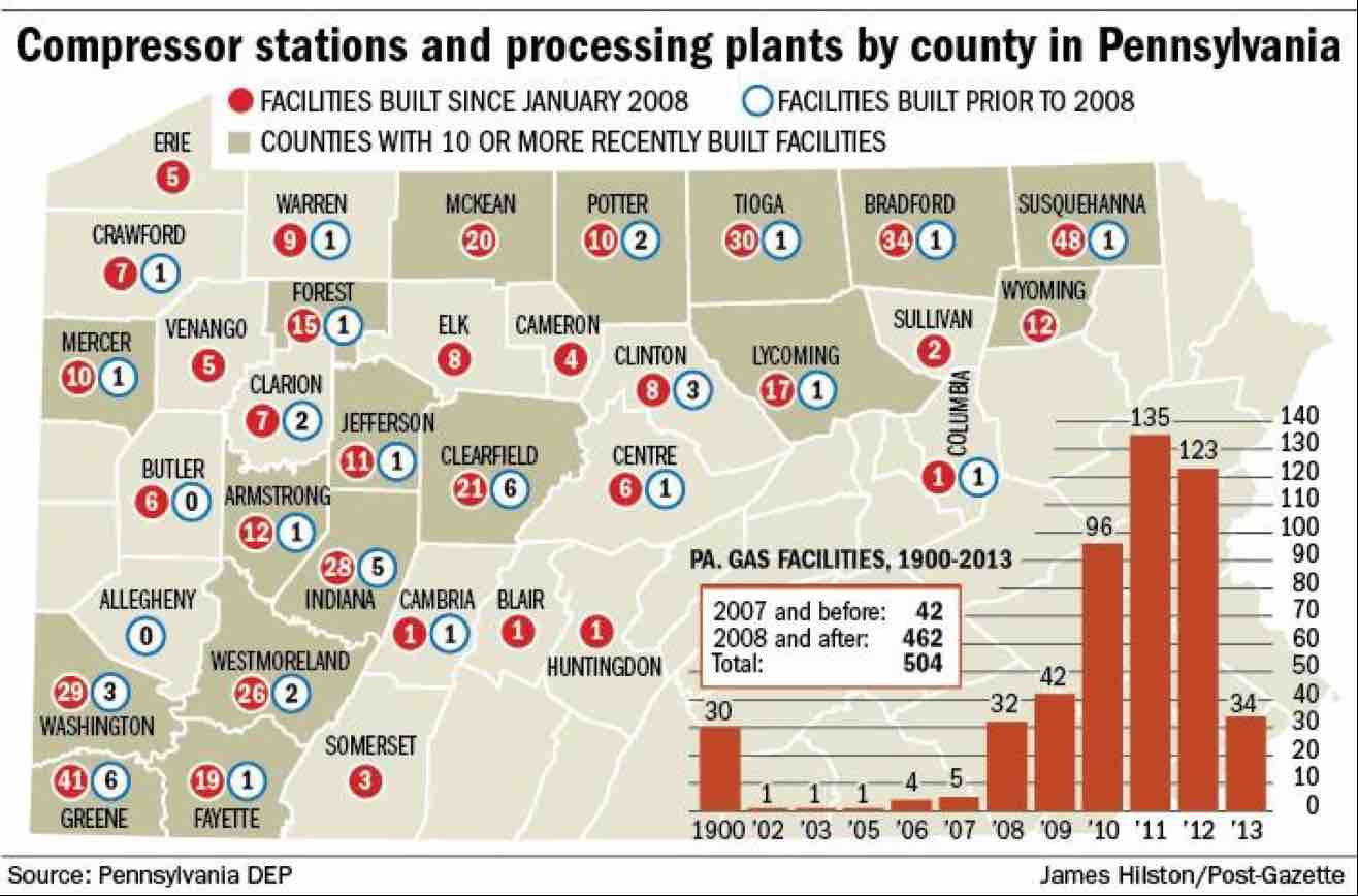
Figure 5. Compressor Stations prior to 2008 and in around 2013. Source: Copied from article by James Hilton in Pittsburgh Post-Gazette.
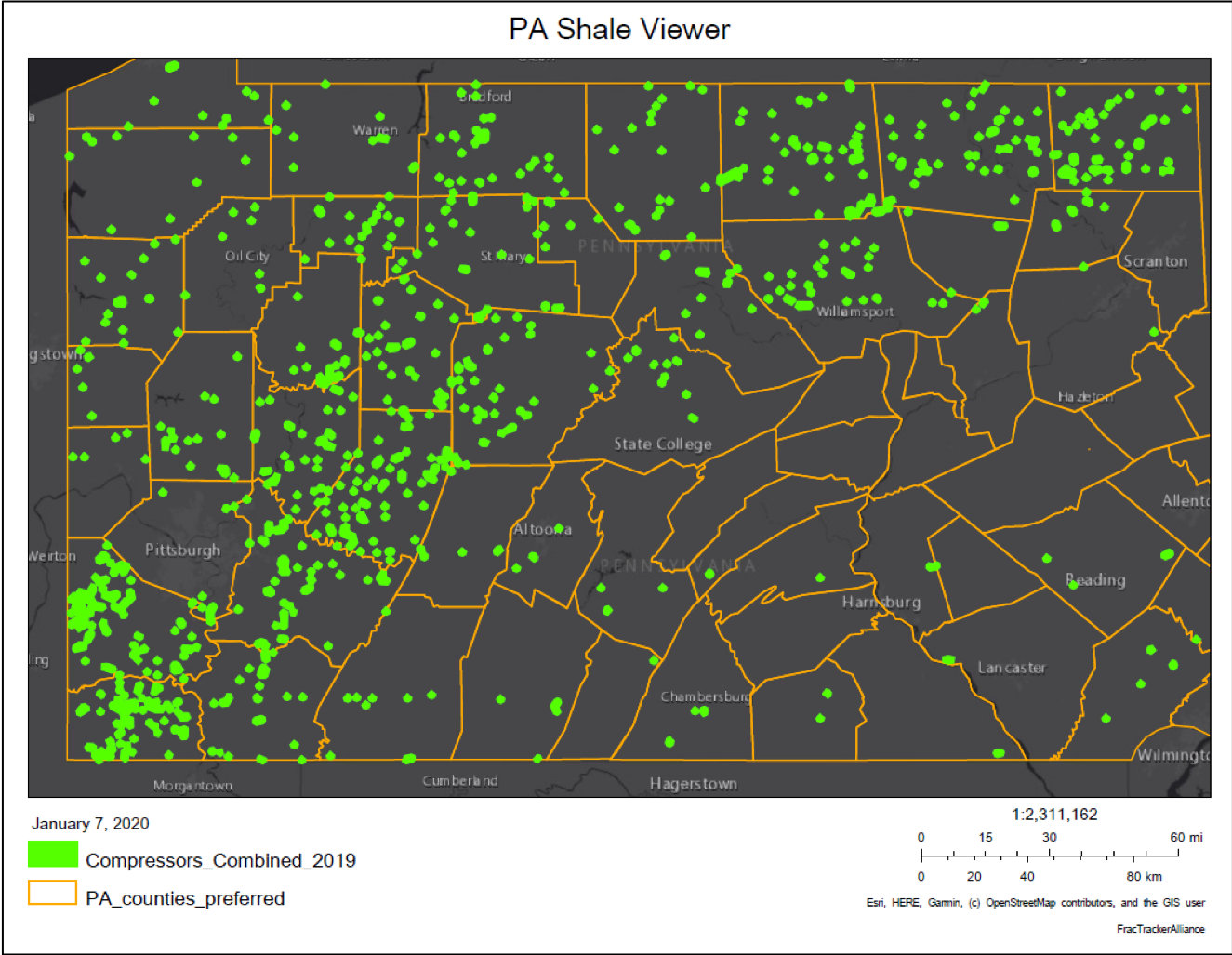
Figure 6. Compressor Stations in Pennsylvania mapped in 2019. Source: FracTracker Alliance. 2000.
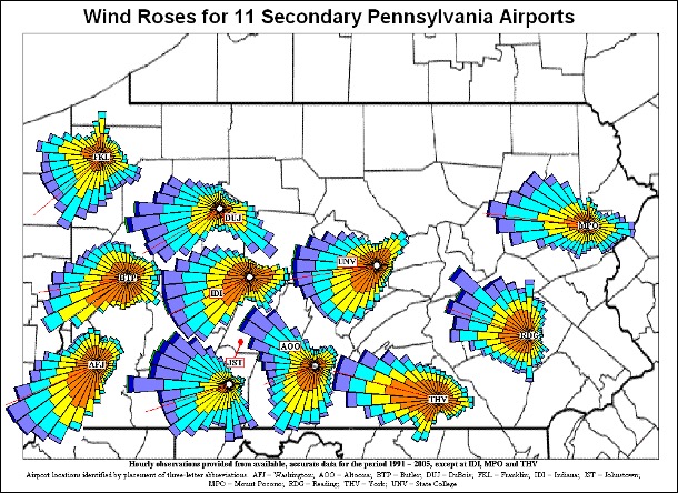
Figure 7. Wind patterns at small airports around Pennsylvania 1991-2005 showing predominant direction of wind and velocity in knots (Orange 0 – 4, Yellow 4 – 7, Turquoise 7 – 11, Medium Blue 11 – 17, Dark Blue 17 – 21). Source: The Pennsylvania State Climatologist.
As permanent, constant sources of air and noise pollution and safety risks, CS add significant costs to communities. Poor air quality alone is well-established as an economic drain for a region due to many factors including increased health care, lower property values, a declining tax base, and difficulty in attracting new businesses or housing development. Litovitz et al. (2013) estimated that, compared to other activities of shale gas extraction, CS made up the majority of the annual emissions of important air toxins in 2011, and therefore a majority of the damages from air pollution, totaling 4 – 24 million dollars of the 7 – 32 million dollars of the aggregate air pollution damages from gas operations (Table 9).
Litovitz and others recognize that the costs of damages from the gas industry air pollution in 2011 may appear smaller than the state-wide impacts from other industries, such as coal burning power plants and coke production, but that appearance deserves a second look. First, shale gas extraction activities are concentrated in a few regions of Pennsylvania, and local air quality is most relevant to public health and local economics such as property values. Second, emissions from gas extraction in 2011 was only in its early stages in Pennsylvania and shale gas operations will expand greatly unless regulations change, while coal-fired power plants are declining due to the advanced age of most facilities. For example, in Westmoreland County, PA alone there are over 50 CS in 2020, the number currently in the entire state of New York, where unconventional gas development was suspended due, in large part, to concerns for public health. Costs from one aspect of an energy sector can be viewed in the context of economic and other benefits of alternative energy efforts. For example, Jacobson et al. (2013) estimated that shifting to clean, renewable energy in NY state would prevent 4000 premature deaths each year and save $33 billion/year through air pollution reductions that impact health care, crop production and other costs. Jacobson et al. used government data in their models regarding health benefits and also identified substantial job growth during and after the transition away from fossil fuels toward renewable energy. Pennsylvania has the potential to attain similar benefits in air quality, public health, savings and job growth gained from a shift to clean, renewable energy in place of fossil fuels.
Table 9. a) Emissions from shale gas industry in 2011 throughout Pennsylvania in metric tons per year. b) Costs of damages due to air pollution from shale gas extraction in 2011 throughout Pennsylvania. Copied from Tables 5 and 6 in Litovitz et al. 2013.
a)
| Activities | VOC | NOx | PM2.5 | PM10 | SOx |
| (1) Transport | 31–54 | 550–1000 | 16–30 | 17–30 | 0.82–1.4 |
| (2) Well drilling and hydraulic fracturing | 260–290 | 6600–8100 | 150–220 | 150–220 | 6.6–190 |
| (3) Production | 71–1800 | 810–1000 | 15–78 | 15–78 | 4.8–6.2 |
| (4) Compressor stations | 2200–8900 | 9300–18 000 | 280–1100 | 280–1100 | 0–340 |
| Totalᵃ | 2500–11 000 | 17 000–28 000 | 460–1400 | 460–1400 | 12–540 |
ᵃ These totals are reported to two significant figures, as are all intermediate emissions values in this document. The activity emissions may not exactly sum to the totals.
b)
| Activities | Timeframe | Total regional damage for 2011 ($2011) | Average per well or per MMCF damage ($2011) |
| (1) Transport | Development | $320 000–$810 000 | $180–$460 per well |
| (2) Well drilling, fracturing | Development | $2 200 000–$4 700 0 | $1 200-$2 700 per well |
| (3) Production | Ongoing | $290 000–$2 700 0 | $0.27-$2.60 per MMCF |
| (4) Compressor stations | Ongoing | $4 400 000–$24 000 000 | $4.20-$23.00 per MMCF |
| (1)-(4) Aggregated | Both | $7 200 000–$32 000 000 | NA |
Brown, David, Celia Lewis, Beth I. Weinberger and Heather Bonaparte. 2014. Understanding air exposure from natural gas drilling put air standards to the test. Reviews in Environmental Health. https://doi.org/10.1515/reveh-2014-0002
Brown, David, Celia Lewis and Beth I. Weinberger. 2015. Human exposure to unconventional natural gas development; a public health demonstration of high exposure to chemical mixtures in ambient air. Journal of Environmental Science and Health (Part A) 50: 460-472.
Ciencewicki, J. and I. Jaspers 2007. Air Pollution and Respiratory Viral Infection. Inhalation Toxicology 19:1135–1146, DOI: https://doi.org/10.1080/08958370701665434
Currie, J, M Greenstone and K Meckel. 2017. Hydraulic fracturing and infant health: New evidence from Pennsylvania. Science Advances 2017;3:e1603021
Eastern Research Group, Inc. and Sage Environmental Consulting, LP. City of Fort Worth natural gas air quality study: final report. July 13, 2011. http://fortworthtexas.gov/gaswells/air-quality-study/final/
Goetz, J.D. E. Floerchinger, E., C. Fortner, J. Wormhoudt, P. Massoli, W. Berk Knighton, S.C. Herndon, C.E. Kolb, E. Knipping, S. L. Shaw, and P. F. DeCarlo. 2015. Atmospheric Emission Characterization of Marcellus Shale Natural Gas Development Sites. Environ. Sci. Technol. 49, 7012−7020. DOI: https://doi.org/10.1021/acs.est.5b00452
Jacobson, MZ, RW Howarth, MA Delucchi, ST Scobie, JH Barth, M Dvorak, M Klevze, H. Hatkhuda, B. Mirand, NA Chowdhury, R Jones, L Plano, AR Ingraffea. 2013. Examining the feasibility of converting New York State’s all-purpose energy infrastructure to one using wind, water, and sunlight. Energy Policy 57: 585-601.
Litovitz, A., A. Curtright, S. Abramzon, N. Burger and C. Samaras. 2013. Estimation of regional air-quality damages from Marcellus Shale natural gas extraction in Pennsylvania. Environ. Res. Lett. 8; 014017 (8pp) doi:10.1088/1748-9326/8/1/014017. https://iopscience.iop.org/article/10.1088/1748-9326/8/1/014017/meta
Macey, G.P., Breech, R., Chernaik, M. (2014) Air concentrations of volatile compounds near oil and gas production: a community-based exploratory study. Environ Health 13, 82 (2014). https://doi.org/10.1186/1476-069X-13-82
McKenzie, LM, G Ruisin, RZ Witter, DA Savitz, LS Newman, JL Adgate. 2014. Birth Outcomes and Maternal Residential Proximity to Natural Gas Development in Rural Colorado. Environmental Health Perspectives Vol 22. http://dx.doi.org/10.1289/ehp.1306722.
Nathan BJ, LM Golston, AS O’Brien , K Ross, WA Harrison, L Tao, DJ Larry, DR Johnson, AN Covington, NN Clark, MA Zondlo. 2015. Environ Sci Technol. 2015 Near-Field Characterization of Methane Emission Variability from a Compressor Station Using a Model Aircraft. Environ Sci Technol. 2015 Jul 7;49(13):7896-903 doi: 10.1021/acs.est.5b00705.
Payne, RA, P Wicker, ZL Hildenbrand, DD Carlton, and KA Schug. 2017. Characterization of methane plumes downwind of natural gas compressor stations in Pennsylvania and New York. Science of The Total Environment 580:1214-1221
Russo, PN and DO Carpenter 2017. Health Effects Associated with Stack Chemical Emissions from NYS Natural Gas Compressor Stations: 2008-2014 Institute for Health and the Environment, A Pan American Health Organization / World Health Organization Collaborating Centre in Environmental Health, University at Albany, 5 University Place, Rensselaer New York. Https://www.albany.edu/about/assets/Complete_report.pdf
Saunders, P.J., D. McCoy. R. Goldstein. A. T. Saunders and A. Munroe. 2018. A review of the public health impacts of unconventional natural gas development Environ Geochem Health 40:1–57. https://doi.org/10.1007/s10653-016-9898-x
Compressor Stations in Westmoreland Co. PA in Dec 2019, based on information from FracTracker Alliance, Pennsylvania Department of Environmental Protection Air Quality Report, and the Department of Homeland Security.
| ID # | Facility # | Name/Operator | Municipality | Latitude | Longitude | Status |
| 627743 | 645570 | CNX GAS CO/HICKMAN COMP STA | Bell Twp | 40.5174 | -79.5498 | Active |
| 693305 | 696606 | PEOPLES TWP/RUBRIGHT COMP STA | Bell Twp | 40.5278 | -79.5561 | Active |
| 626482 | 644726 | CNX GAS CO/BELL POINT COMP STA | Bell Twp | 40.5413 | -79.5338 | Active |
| na | na | NORTH OAKFORD | Delmont | 40.4018 | -79.5597 | Active |
| 714057 | 713241 | RW GATHERING LLC/ECKER BERGMAN RD COMP STA | Derry Twp | 40.3533 | -79.3028 | Active |
| 760724 | 752063 | RE GAS DEV/ORGOVAN COMP STA | Derry Twp | 40.3857 | -79.4019 | Active |
| 736807 | 732436 | RW GATHERING LLC/SALEM COMP STA | Derry Twp | 40.3908 | -79.3361 | Active |
| 714057 | 713241 | RW GATHERING LLC/ECKER BERGMAN RD COMP STA | Derry Twp | 40.3533 | -79.3028 | Active |
| 774714 | 766854 | EQT GATHERING LLC/DERRY COMP STA | Derry Twp | 40.4511 | -79.3161 | Active |
| na | na | Layman Compressor, Range Resources Appalachia, LLC | East Huntingdon | 40.1113 | -79.6345 | Unknown |
| na | na | Key Rock Energy/LLC | East Huntingdon | 40.1228 | -79.6489 | Unknown |
| 662759 | 673466 | Kriebel Minerals Inc./Sony Compressor Station (Inactive) | East Huntingdon | 40.181 | -79.5882 | Unknown |
| 662781 | 673477 | Lynn Compressor, Kriebel Minerals Inc. | East Huntingdon | 40.1798 | -79.5557 | Unknown |
| 636316 | 660570 | Range Resources Appalachia/ Layman Compressor Station | East Huntingdon | 40.1086 | -79.6359 | Unknown |
| na | na | Keyrock Energy LLC/ Hribal Compresor Station, East Huntingdon, Pa. (active) | East Huntingdon | 40.1353 | -7905653 | Unknown |
| 761545 | 752755 | KeyRock Energy LLC/ Hribal Compressor Station (Active) | East Huntingdon | 40.1333 | -79.55 | Unknown |
| 649767 | 663499 | Range Resources Appalachia/Schwartz Comp. Station | East Huntingdon | 40.0879 | -79.601 | Unknown |
| 652968 | 665874 | TEXAS KEYSTONE/FAIRFIELD TWP COMP STA | Fairfield Twp | 40.3363 | -79.1786 | Active |
| 557780 | 572987 | EQUITRANS LP/W FAIRFIELD COMP STA | Fairfield Twp | 40.3333 | -79.1167 | Active |
| 675937 | 683303 | DIVERSIFIED OIL & GAS LLC/MURPHY COMP SITE | Fairfield Twp | 40.3362 | -79.1122 | Active |
| 812881 | 806928 | TEXAS KEYSTONE INC/ MURPHY COMP STA | Fairfield Twp | 40.3543 | -79.1123 | Active |
| na | na | SOUTH OAKFORD/Dominion | Greensburg | 40.365 | -79.5585 | Unknown |
| na | na | OAKFORD | Greensburg | 40.3848 | -79.5489 | Active |
| na | na | DELMONT | Geensburg | 40.382 | -79.5554 | Active |
| 496667 | 626720 | Silvis Compressor Station, Exco Resources Pa. Inc | Hempfield | 40.2022 | -79.5526 | Unknown |
| na | na | Dominion Trans Inc., Lincoln Heights | Hempfield Township | 40.3004 | -79.6193 | Active |
| 812660 | 806731 | CNX Gas Co. LLC | Hempfield Township | 40.2957 | -79.6277 | Active |
| 812661 | 806732 | CNX Gas Co. LLC/ Jackson Compressor Station, Status: Active | Hempfield Township | 40.2931 | -79.6119 | Unknown |
| 601521 | 626775 | PEOPLES NATURAL GAS CO/ARNOLD COMP STA | Lower Burrell City | 40.3623 | -79.4316 | Active |
| 812883 | 806930 | TEXAS KEYSTONE INC/LOYALHANNA | Loyalhanna Twp | 40.4514 | -79.4727 | Inactive |
| na | na | J.B. TONKIN | Murrysville Boro | 40.4629 | -79.6402 | Active |
| 815083 | 809310 | HUNTLEY & HUNTLEY INC/BOARST COMP STA | Murrysville Boro | 40.4686 | -79.6417 | Inactive |
| 735725 | 731655 | MTN GATHERING LLC/10078 MAINLINE COMP STA | Murrysville Boro | 40.4708 | -79.65 | Active |
| 241708 | 276314 | Dominion Trans Inc/Jeannette | Penn Township | 40.3317 | -79.5935 | inactive |
| na | 701239 | DOMINION ENERGY TRANS INC/ROCK SPRINGS COMP STA | Salem Twp | 40.4052 | -79.5546 | Unknown |
| na | na | OAKFORD | Salem Twp | 40.4052 | -79.5546 | Unknown |
| 465965 | 495182 | EQT GATHERING/SLEEPY HOLLOW COMP STA | Salem Twp | 40.3634 | -79.5426 | Inactive |
| 465965 | 495182 | EQT GATHERING/SLEEPY HOLLOW COMP STA | Salem Twp | 40.3634 | -79.5426 | Inactive |
| 483173 | 512126 | COLUMBIA GAS TRANS CORP/DELMONT COMP STA | Salem Twp | 40.3871 | -79.5638 | Active |
| 707759 | 708010 | LAUREL MTN MIDSTREAM OPR LLC/SALEM COMP STA | Salem Twp | 40.3782 | -79.4929 | Active |
| 459024 | 488214 | CNX Gas Co./ Jacobs Creek Compressor Station, | South Huntingdon Twp | 40.1172 | -79.6681 | Unknown |
| 634559 | 650802 | Rex Energy I LLC/Launtz | Unity Twp | 40.3325 | -79.4295 | Unknown |
| na | 668776 | Keyrock Energy LLC/ Unity Compressor Station | Unity Twp | 40.2251 | -79.5109 | Unknown |
| na | na | Nelson/RE Gas Dev LLC | UnityTwp | 40.3378 | -79.4348 | Unknown |
| 657366 | 66932 | People’s Natural Gas/ Latrobe Compressor Station | Unity Twp | 40.3075 | -79.4369 | Inactive |
| 812662 | 806733 | CNX Gas Co. LLC, Troy Compressor Station | Unity Twp | na | na | Unknown |
| 657366 | 564168 | Dominion Peoples (Inactive) | Unity Twp | 40.3073 | -79.4371 | Inactive |
| 815196 | 809457 | HUNTLEY & HUNTLEY INC/WASHINGTON STATION | Washington Twp | 40.4967 | -79.6206 | Active |
| 605562 | 629821 | PEOPLES NATURAL GAS/MERWIN COMP STA | Washington Twp | 40.5083 | -79.6203 | Active |
| 815203 | 809466 | HUNTLEY & HUNTLEY INC/TARPAY STA | Washington Twp | 40.5222 | -79.6186 | Active |
| na | na | Mamont (CNX GAS CO/MAMONT COMP STA) | Washington Twp | 40.5046 | -79.5862 | Unkown |
| 741197 | 735870 | CONE MIDSTREAM PARTNERS LP/MAMONT COMP STA | Washington Twp | 40.5067 | -79.5644 | Active |
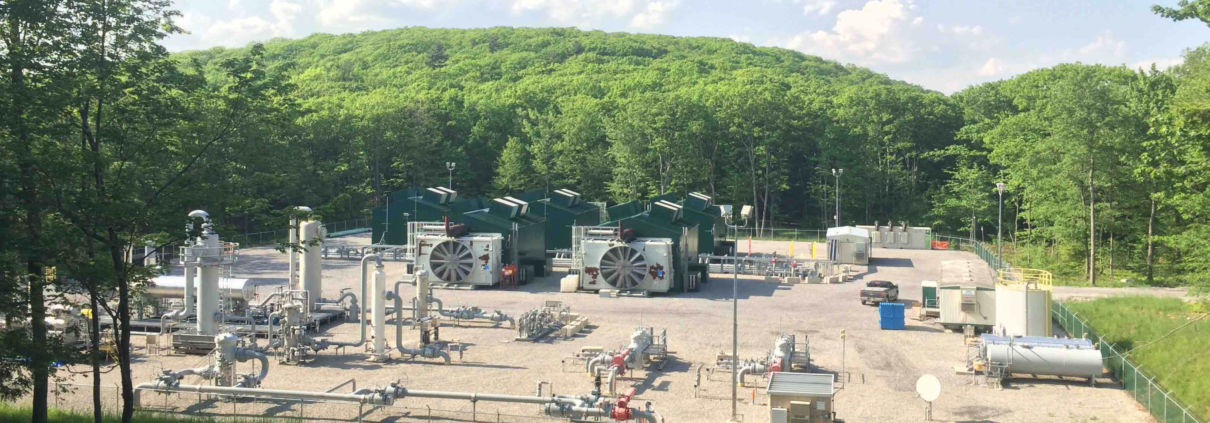
Feature image of a compressor station within Loyalsock State Forest, PA. Photo by Brook Lenker, FracTracker Alliance, June 2016.
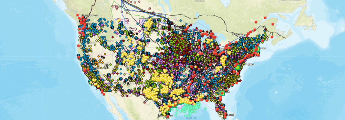
FracTracker Alliance has released a new national map, filled with energy and petrochemical data. Explore the map, continue reading to learn more, and see how your state measures up!
This map has been updated since this blog post was originally published, and therefore statistics and figures below may no longer correspond with the map
The items on the map (followed by facility count in parenthesis) include:
For oil and gas wells, view FracTracker’s state maps.
This map is by no means exhaustive, but is exhausting. It takes a lot of infrastructure to meet the energy demands from industries, transportation, residents, and businesses – and the vast majority of these facilities are powered by fossil fuels. What can we learn about the state of our national energy ecosystem from visualizing this infrastructure? And with increasing urgency to decarbonize within the next one to three decades, how close are we to completely reengineering the way we make energy?
The “power plant” legend item on this map contains facilities with an electric generating capacity of at least one megawatt, and includes independent power producers, electric utilities, commercial plants, and industrial plants. What does this data reveal?
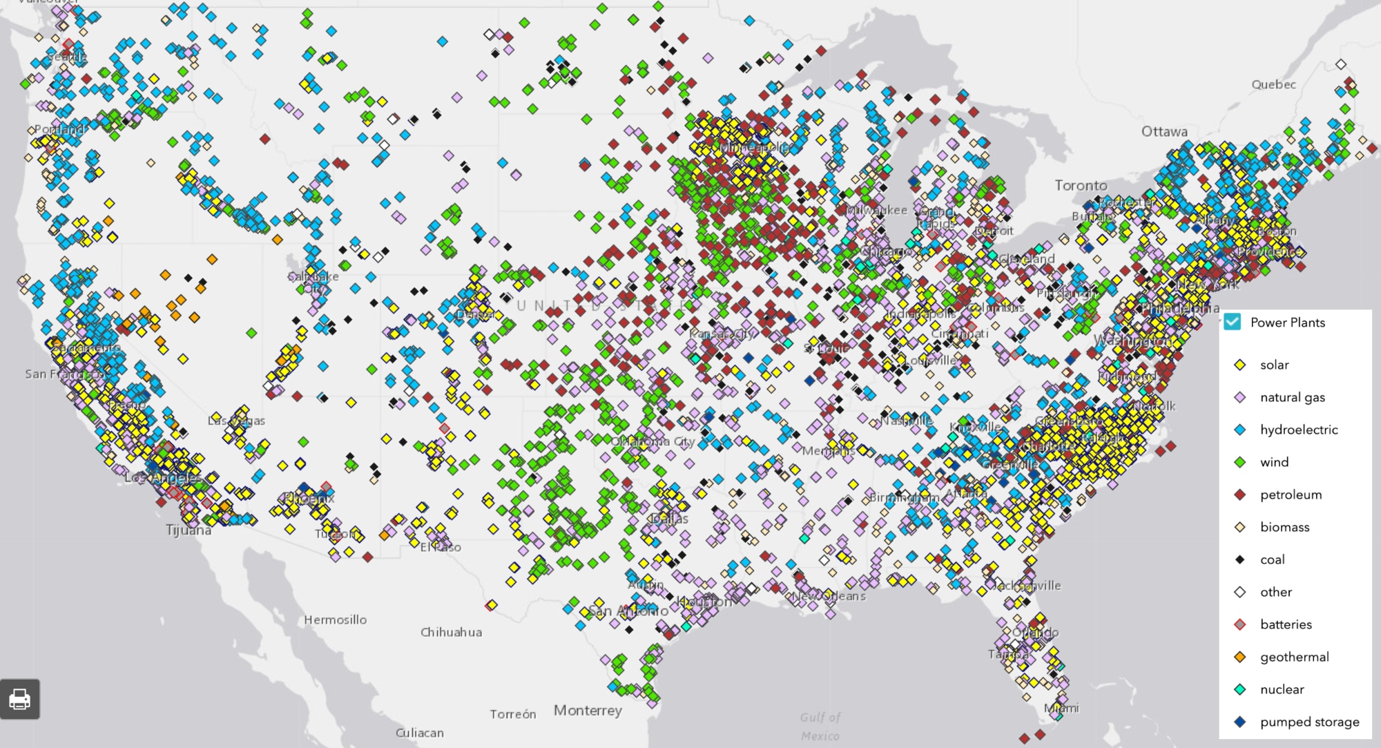
Power plants by energy source. Data from EIA.
In terms of the raw number of power plants – solar plants tops the list, with 2,916 facilities, followed by natural gas at 1,747.
In terms of megawatts of electricity generated, the picture is much different – with natural gas supplying the highest percentage of electricity (44%), much more than the second place source, which is coal at 21%, and far more than solar, which generates only 3% (Figure 1).
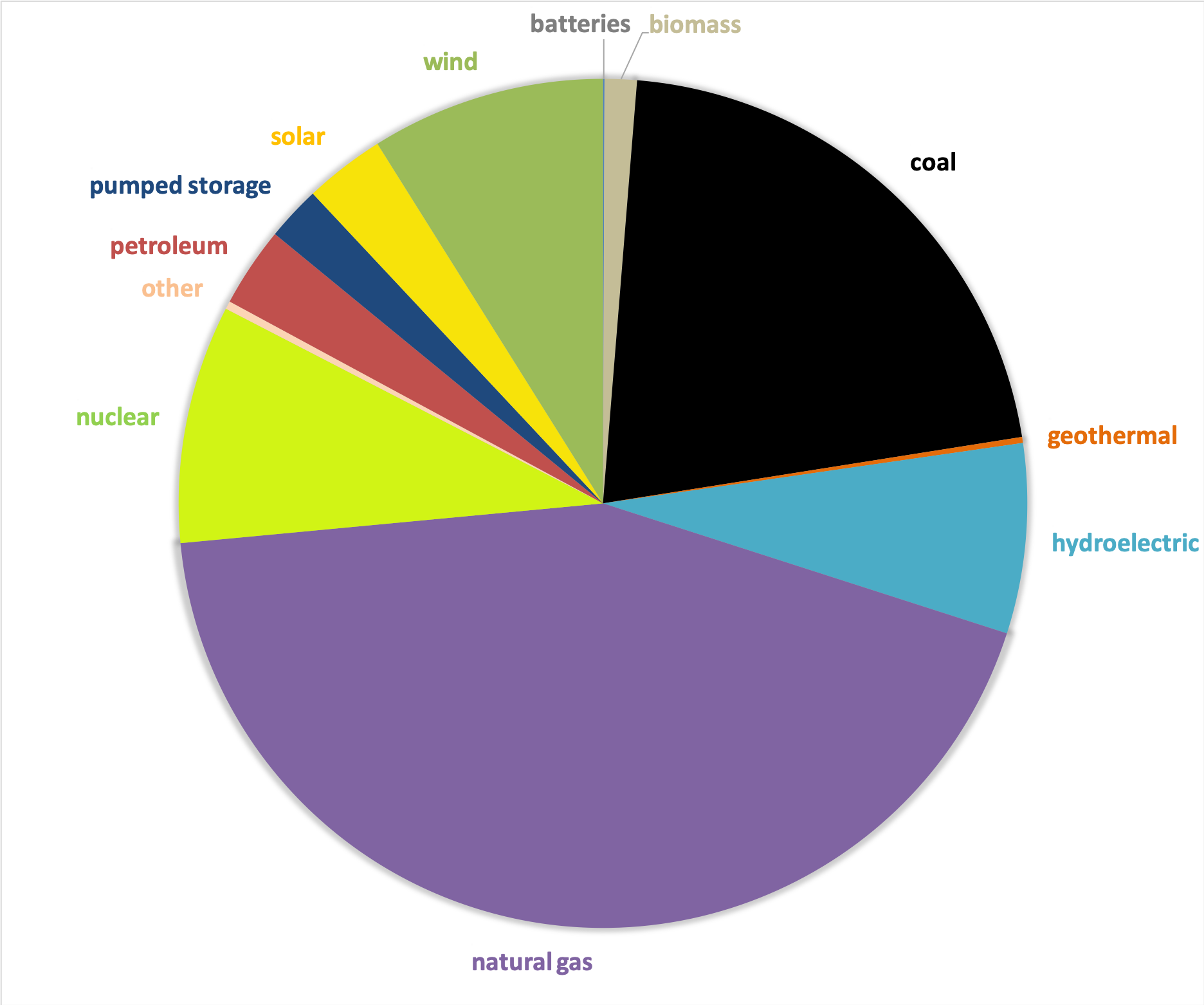
Figure 1. Electricity generation by source in the United States, 2019. Data from EIA.
This difference speaks to the decentralized nature of the solar industry, with more facilities producing less energy. At a glance, this may seem less efficient and more costly than the natural gas alternative, which has fewer plants producing more energy. But in reality, each of these natural gas plants depend on thousands of fracked wells – and they’re anything but efficient.
The cost per megawatt hour of electricity for a renewable energy power plants is now cheaper than that of fracked gas power plants. A report by the Rocky Mountain Institute, found “even as clean energy costs continue to fall, utilities and other investors have announced plans for over $70 billion in new gas-fired power plant construction through 2025. RMI research finds that 90% of this proposed capacity is more costly than equivalent [clean energy portfolios, which consist of wind, solar, and energy storage technologies] and, if those plants are built anyway, they would be uneconomic to continue operating in 2035.”
The economics side with renewables – but with solar, wind, geothermal comprising only 12% of the energy pie, and hydropower at 7%, do renewables have the capacity to meet the nation’s energy needs? Yes! Even the Energy Information Administration, a notorious skeptic of renewable energy’s potential, forecasted renewables would beat out natural gas in terms of electricity generation by 2050 in their 2020 Annual Energy Outlook.
This prediction doesn’t take into account any future legislation limiting fossil fuel infrastructure. A ban on fracking or policies under a Green New Deal could push renewables into the lead much sooner than 2050.
In a void of national leadership on the transition to cleaner energy, a few states have bolstered their renewable portfolio.
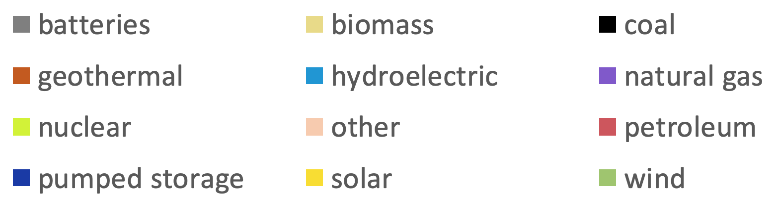
Figure 2. Electricity generation state-wide by source, 2019. Data from EIA.
One final factor to consider – the pie pieces on these state charts aren’t weighted equally, with some states’ capacity to generate electricity far greater than others. The top five electricity producers are Texas, California, Florida, Pennsylvania, and Illinois.
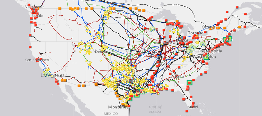
In 2018, approximately 28% of total U.S. energy consumption was for transportation. To understand the scale of infrastructure that serves this sector, it’s helpful to click on the petroleum refineries, crude oil rail terminals, and crude oil pipelines on the map.
Transportation Fuel Infrastructure. Data from EIA.
The majority of gasoline we use in our cars in the US is produced domestically. Crude oil from wells goes to refineries to be processed into products like diesel fuel and gasoline. Gasoline is taken by pipelines, tanker, rail, or barge to storage terminals (add the “petroleum product terminal” and “petroleum product pipelines” legend items), and then by truck to be further processed and delivered to gas stations.
The International Energy Agency predicts that demand for crude oil will reach a peak in 2030 due to a rise in electric vehicles, including busses. Over 75% of the gasoline and diesel displacement by electric vehicles globally has come from electric buses.
China leads the world in this movement. In 2018, just over half of the world’s electric vehicles sales occurred in China. Analysts predict that the country’s oil demand will peak in the next five years thanks to battery-powered vehicles and high-speed rail.
In the United States, the percentage of electric vehicles on the road is small but growing quickly. Tax credits and incentives will be important for encouraging this transition. Almost half of the country’s electric vehicle sales are in California, where incentives are added to the federal tax credit. California also has a “Zero Emission Vehicle” program, requiring electric vehicles to comprise a certain percentage of sales.
We can’t ignore where electric vehicles are sourcing their power – and for that we must go back up to the electricity generation section. If you’re charging your car in a state powered mainly by fossil fuels (as many are), then the electricity is still tied to fossil fuels.
Many of the oil and gas infrastructure on the map doesn’t go towards energy at all, but rather aids in manufacturing petrochemicals – the basis of products like plastic, fertilizer, solvents, detergents, and resins.
This industry is largely concentrated in Texas and Louisiana but rapidly expanding in Pennsylvania, Ohio, and West Virginia.
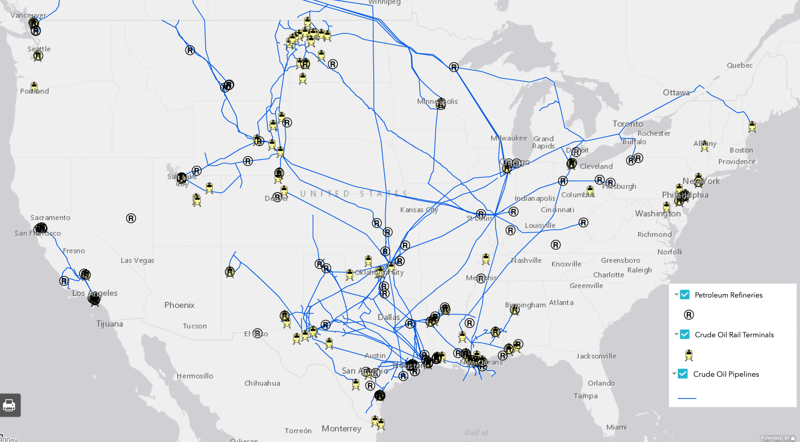
On this map, key petrochemical facilities include natural gas plants, chemical plants, ethane crackers, and natural gas liquid pipelines.
Petrochemical infrastructure. Data from EIA.
Natural gas processing plants separate components of the natural gas stream to extract natural gas liquids like ethane and propane – which are transported through the natural gas liquid pipelines. These natural gas liquids are key building blocks of the petrochemical industry.
Ethane crackers process natural gas liquids into polyethylene – the most common type of plastic.
The chemical plants on this map include petrochemical production plants and ammonia manufacturing. Ammonia, which is used in fertilizer production, is one of the top synthetic chemicals produced in the world, and most of it comes from steam reforming natural gas.
As we discuss ways to decarbonize the country, petrochemicals must be a major focus of our efforts. That’s because petrochemicals are expected to account for over a third of global oil demand growth by 2030 and nearly half of demand growth by 2050 – thanks largely to an increase in plastic production. The International Energy Agency calls petrochemicals a “blind spot” in the global energy debate.
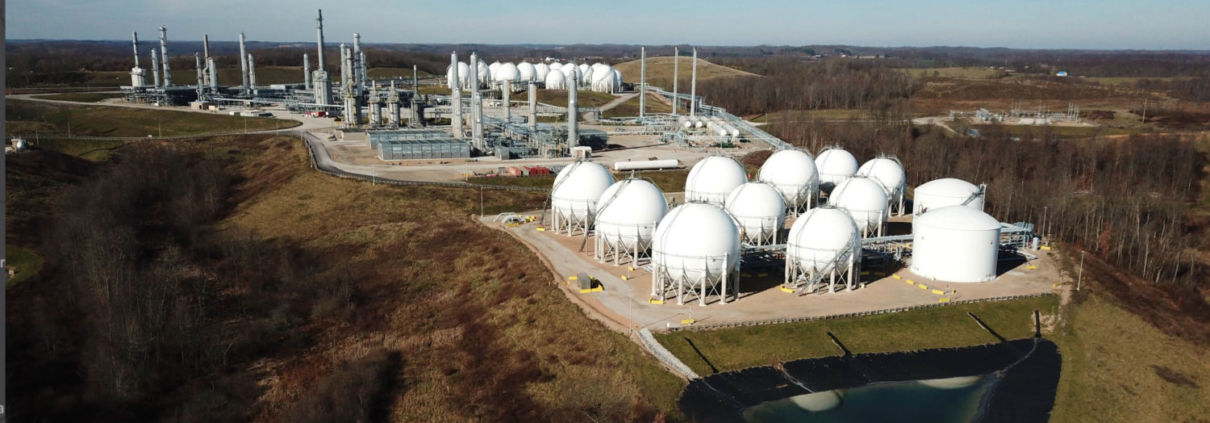
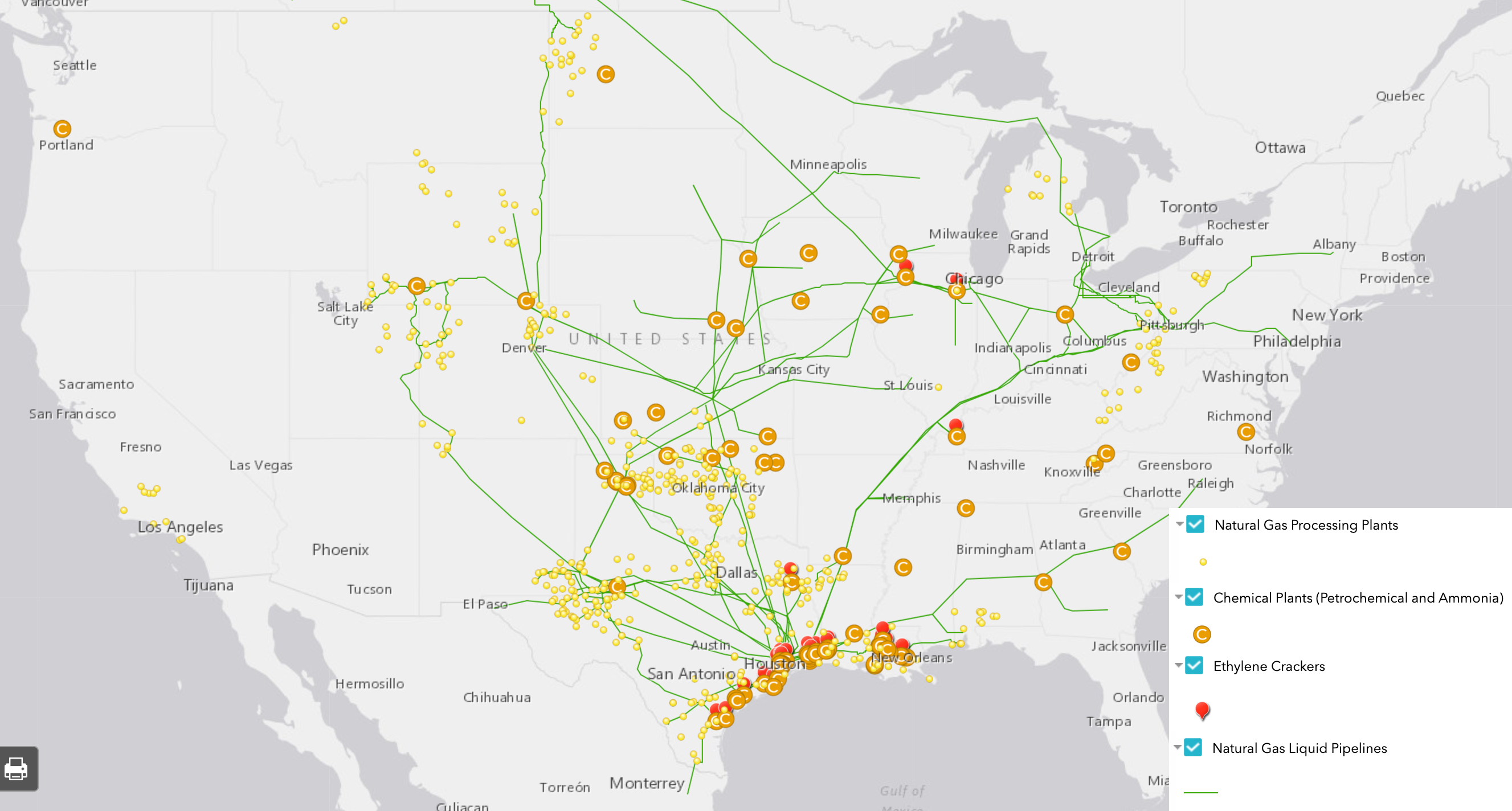
Petrochemical development off the coast of Texas, November 2019. Photo by Ted Auch, aerial support provided by LightHawk.
Investing in plastic manufacturing is the fossil fuel industry’s strategy to remain relevant in a renewable energy world. As such, we can’t break up with fossil fuels without also giving up our reliance on plastic. Legislation like the Break Free From Plastic Pollution Act get to the heart of this issue, by pausing construction of new ethane crackers, ensuring the power of local governments to enact plastic bans, and phasing out certain single-use products.
Mapped out, this web of fossil fuel infrastructure seems like a permanent grid locking us into a carbon-intensive future. But even more overwhelming than the ubiquity of fossil fuels in the US is how quickly this infrastructure has all been built. Everything on this map was constructed since Industrial Revolution, and the vast majority in the last century (Figure 3) – an inch on the mile-long timeline of human civilization.
Figure 3. Global Fossil Fuel Consumption. Data from Vaclav Smil (2017)
In fact, over half of the carbon from burning fossil fuels has been released in the last 30 years. As David Wallace Wells writes in The Uninhabitable Earth, “we have done as much damage to the fate of the planet and its ability to sustain human life and civilization since Al Gore published his first book on climate than in all the centuries—all the millennia—that came before.”
What will this map look like in the next 30 years?
A recent report on the global economics of the oil industry states, “To phase out petroleum products (and fossil fuels in general), the entire global industrial ecosystem will need to be reengineered, retooled and fundamentally rebuilt…This will be perhaps the greatest industrial challenge the world has ever faced historically.”
Is it possible to build a decentralized energy grid, generated by a diverse array of renewable, local, natural resources and backed up by battery power? Could all communities have the opportunity to control their energy through member-owned cooperatives instead of profit-thirsty corporations? Could microgrids improve the resiliency of our system in the face of increasingly intense natural disasters and ensure power in remote regions? Could hydrogen provide power for energy-intensive industries like steel and iron production? Could high speed rail, electric vehicles, a robust public transportation network and bike-able cities negate the need for gasoline and diesel? Could traditional methods of farming reduce our dependency on oil and gas-based fertilizers? Could zero waste cities stop our reliance on single-use plastic?
Of course! Technology evolves at lightning speed. Thirty years ago we didn’t know what fracking was and we didn’t have smart phones. The greater challenge lies in breaking the fossil fuel industry’s hold on our political system and convincing our leaders that human health and the environment shouldn’t be externalized costs of economic growth.
For Immediate Release
Contact: Lee Ziesche, lee@saneenergyproject.org, 954-415-6282
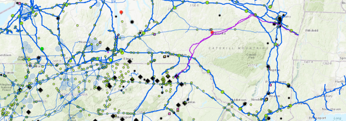
Interactive Map Shows Expansion of Fracked Gas Infrastructure in New York State
And showcases powerful community resistance to it
New York, NY – A little over a year after 55 New Yorkers were arrested outside of Governor Cuomo’s door calling on him to be a true climate leader and halt the expansion of fracked gas infrastructure in New York State, grassroots advocates Sane Energy Project re-launched the You Are Here (YAH) map, an interactive map that shows an expanding system of fracked infrastructure approved by the Governor.
“When Governor Cuomo announced New York’s climate goals in early 2019, it’s clear there is no room for more extractive energy, like fossil fuels.” said Kim Fraczek, Director of Sane Energy Project, “Yet, I look at the You Are Here Map, and I see a web of fracked gas pipelines and power plants trapping communities, poisoning our water, and contributing to climate change.”
Sane Energy originally launched the YAH map in 2014 on the eve of the historic People’s Climate March, and since then, has been working with communities that resist fracked gas infrastructure to update the map and tell their stories.
“If you read the paper, you might think Governor Cuomo is a climate leader, but one look at the YAH Map and you know that isn’t true. Communities across the state are living with the risks of Governor Cuomo’s unprecedented buildout of fracked gas infrastructure,” said Courtney Williams, a mother of two young children living within 400 feet of the AIM fracked gas pipeline. “The Governor has done nothing to address the risks posed by the “Algonquin” Pipeline running under Indian Point Nuclear Power Plant. That is the center of a bullseye that puts 20 million people in danger.”
Fracked gas infrastructure poses many of the same health risks as fracking and the YAH map exposes a major hypocrisy when it comes to Governor Cuomo’s environmental credentials. The Governor has promised a Green New Deal for New York, but climate science has found the expansion of fracking and fracked gas infrastructure is increasing greenhouse gas emissions in the United States.
“The YAH map has been an invaluable organizing tool. The mothers I work with see the map and instantly understand how they are connected across geography and they feel less alone. This solidarity among mothers is how we build our power ,” said Lisa Marshall who began organizing with Mothers Out Front to oppose the expansion of the Dominion fracked gas pipeline in the Southern Tier and a compressor station built near her home in Horseheads, New York. “One look at the map and it’s obvious that Governor Cuomo hasn’t done enough to preserve a livable climate for our children.”
“Community resistance beat fracking and the Constitution Pipeline in our area,” said Kate O’Donnell of Concerned Citizens of Oneonta and Compressor Free Franklin. “Yet smaller, lesser known infrastructure like bomb trucks and a proposed gas decompressor station and 25 % increase in gas supply still threaten our communities.”
The YAH map was built in partnership with FracTracker, a non-profit that shares maps, images, data, and analysis related to the oil and gas industry hoping that a better informed public will be able to make better informed decisions regarding the world’s energy future.
“It has been a privilege to collaborate with Sane Energy Project to bring our different expertise to visualizing the extent of the destruction from the fossil fuel industry. We look forward to moving these detrimental projects to the WINS layer, as communities organize together to take control of their energy future. Only then, can we see a true expansion of renewable energy and sustainable communities,” said Karen Edelstein, Eastern Program Coordinator at Fractracker Alliance.
Throughout May and June Sane Energy Project and 350.org will be traveling across the state on the ‘Sit, Stand Sing’ tour to communities featured on the map to hold trainings on nonviolent direct action and building organizing skills that connect together the communities of resistance.
“Resistance to fracking infrastructure always starts with small, volunteer led community groups,” said Lee Ziesche, Sane Energy Community Engagement Coordinator. “When these fracked gas projects come to town they’re up against one of the most powerful industries in the world. The You Are Here Map and ‘Sit, Stand Sing’ tour will connect these fights and help build the power we need to stop the harm and make a just transition to community owned renewable energy.”
Last month, FracTracker Alliance featured a blog entry and map exploring the controversy around National Fuel’s proposed Northern Access Pipeline (NAPL) project, shown in the map below. The proposed project, which has already received approval from the Federal Energy Regulatory Commission (FERC), is still awaiting another decision by April 7, 2017 — Section 401 Water Quality Certification. By that date, the New York State Department of Environmental Conservation (NYS DEC) must give either final approval, or else deny the project.
Northern Access Pipeline Map
View map fullscreen | How FracTracker maps work
The NAPL project includes the construction of 97-mile-long pipeline to bring fracked Marcellus gas through New York State, and into Canada. The project also involves construction of a variety of related major infrastructure projects, including a gas dehydration facility, and a ten-fold expansion of the capacity of the Porterville Compressor Station located at the northern terminus of the proposed pipeline, in Erie County, NY.
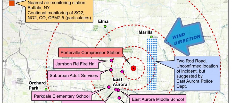
On three consecutive days in early February, 2017, the New York State Department of Environmental Conservation (NYS DEC) held hearings in Western New York to gather input about the NAPL project. On February 7th, the day of the first meeting at Saint Bonaventure University in Allegany County, NY, an alarming — and yet to be fully reported — incident widely considered to be a gas leak, occurred at, or near, the Porterville Compressor Station (also known locally as the “Elma Compressor Station”). The incident is thought to be connected to the planned upgrades to the facility, but was not even mentioned as a concern during the public meetings relating to the Northern Access Pipeline in the subsequent hours and days.
What follows is a story of poor communication between the utility company, first responders, and local residents, resulting in confusion and even panic, and has yet to be conclusively explained to the general public.
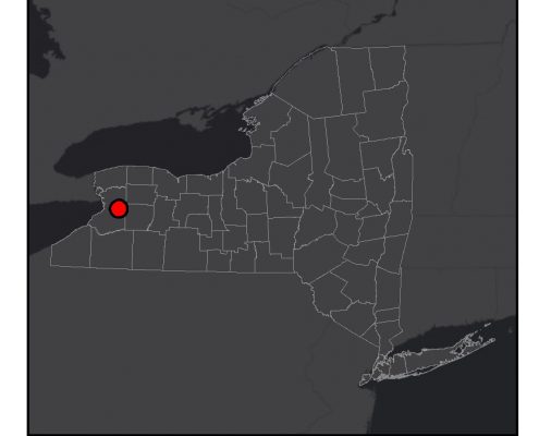
Area of incident in NY State
We know that a little past 10 AM on February 7th, people in the villages of Elma and East Aurora, within about a mile of the Porterville Compressor Station, reported strong odors of gas. They filed complaints with the local gas utility (National Fuel), and the local 911 center, which referred the calls to the local Elma Fire Department. The fire department went to the Porterville Compressor station to investigate, remembering a similar incident from a few years earlier. At the compressor station, representatives from National Fuel, the operator of the compressor station, assured the fire company that they were conducting a routine flushing of an odorant line, and the situation was under control, so the fire company departed.
Residents in the area became more alarmed when they noticed that the odor was stronger outside their buildings than inside them. National Fuel then ordered many residents to evacuate their homes. The East Aurora police facilitated the evacuation and instructed residents to gather in the East Aurora Library not far from those homes. Nearby businesses, such as Fisher Price, headquartered in East Aurora, chose to send their employees home for the day, due to the offensive odor and perceived risks.
Around 11:30 in the morning, up to 200 clients at Suburban Adult Services, Inc. (SASi), were evacuated to the Jamison Road Fire Station, where they remained until around 3 PM that afternoon. Over 200 reports were received, some from as far away as Orchard Park, eight miles down-wind of the compressor station.
After East Aurora elementary and middle schools placed complaints, National Fuel told them to evacuate students and staff from their buildings. Realizing that the smell was stronger outside than inside the building, school leaders revised their plans, and started to get buses ready to transport student to the high school, where there had not been reports of the odor. Before the buses could load, however, the police department notified the school that the gas leak had been repaired, and that there was no need to evacuate. School officials then activated the school’s air circulation system to rid the building of the fumes.
Perplexingly, according to one report, National Fuel’s Communications Manager Karen Merkel said “that the company did not reach out into the community to tell people what was going on because the company cannot discourage anyone from making an emergency gas call.”
Merkel noted further, “You never know if the smell being reported is related to work we are doing or another gas leak,” she said. “This wouldn’t be determined until we investigate it.”
Some background on gas leaks & odorant additives

Ethyl mercaptan molecule
An odorant, such as ethyl mercaptan, is often added to natural gas in order to serve as an “early warning system” in the event of a leak from the system. Odorants like mercaptan are especially effective because the humans can smell very low concentrations of it in the air. According to the National Center for Biotechnology Information, “The level of distinct odor awareness (LOA) for ethyl mercaptan odorant is 1.4 x10⁻⁴ ppm,” or 0.00014 parts per million. That translates to 0.000000014 percent by volume.
Not all natural gas is odorized, however. According to Chevron Phillips, “mercaptans are required (by state and federal regulations) to be added to the gas stream near points of consumption as well as in pipelines that are near areas with certain population density requirements, per Department of Transportation regulations… Not all gas is odorized, though; large industrial users served by transmission lines away from everyday consumers might not be required to use odorized gas.” Also, because odorants tend to degrade or oxidize when gas is travelling a long distance through transmission lines, they are not always added to larger pipeline systems.
The explosion and flammability concentration limit for natural gas refers to the percentage range at which a gas will explode. At very low concentrations, the gas will not ignite. If the concentration is too high, not enough oxygen is present, and the gas is also stable. This is why gas in non-leaky pipelines does not explode, but when it mixes with air, and a spark is present, the result can be disastrous. Methane, the primary component of natural gas, has a lower explosive level (LEL) of 4.4% and an upper explosive limit (UEL) (above which it will not ignite) of 16.4%. Nonetheless, levels above 1% are still worrisome, and may still be good cause for evacuation.
Therefore, the margin of safety between when natural gas is detectable with an odorant present, and when it may explode, is very broad. This may help to explain why the smell of gas was detected over such a broad distance, but no explosion (very fortunately) took place.
Many East Aurora residents have had first-hand experience with the dangers posed by gas lines in their community. Less than 25 years ago, in September 1994, a high-pressure pipeline owned by National Fuel ruptured in an uninhabited area between East Aurora and South Wales along Olean Rd. The blast left a 10-foot-deep, 20-foot-wide crater, and tree limbs and vegetation were burned as far as 50 feet away.
FracTracker spoke extensively with one resident of East Aurora, Jennifer Marmion, about her experiences, and efforts to understand what had actually happened the day of this incident.
When personnel from the Jamison Fire Company — who are assumed to be first responders to emergencies of this sort — arrived at the Porterville Compressor Station, they were told by National Fuel that there was no hazard and that their services were not needed. Consequently, these crews left the site. The East Aurora Police Department was given a different explanation by National Fuel; there was a valve malfunction somewhere along Two Rod Road in Marilla. Still later, National Fuel indicated that the pipeline changeover occurred closer to the compressor station itself. The closest distance between anywhere on Two Rod Road and the compressor station, itself, is a mile and a half. And Ms. Marmion was given a still different story by a National Fuel engineer: that the odor, indeed, resulted during the replacement of a 100-foot-long section of aging pipeline at the Porterville (“Elma”) Compressor Station.
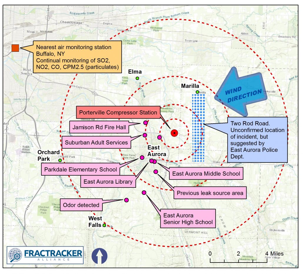
Key locations in incident report
Some reports indicated an alternate explanation: that the odor originated at the East Aurora Town Hall (J. Marmion, pers. comm., via Channel 7 News), or a leaky valve along a pipeline near Marilla (J. Marmion, pers. comm, via East Aurora Police Department dispatcher). A member of the East Aurora Fire Department surmised that the leak might have been closer to Olean Road, south of the village, where there was a history of other leaks. The day after the incident, National Fuel indicated that the odor originated from the compressor station, and was the result of a routine, scheduled “blowdown” by National Fuel — wherein gas lines at the compressor station are cleared as part of routine maintenance. However, when pressed for more details, they did not provide them.
More than six weeks have passed since the incident, and there is still no definitive explanation available. Clearly, there was considerable confusion about what the correct, and safe, procedure needed to be, as well as how this information needed to flow to the public. Ultimately, a representative from National Fuel’s Government Affairs office agreed that he would alert the local towns and fire departments when maintenance activities would be occurring. It is surprising that this was not already standard practice.
Although Ms. Marmion is continuing to be a determined citizen activist, she has been met with a frustrating array of ambiguous and often conflicting descriptions, phone calls that go un-answered, voice mailboxes at offices that are either full or not set up to receive messages. Furthermore, although National Fuel has told Marmion that there is an Action Plan to be followed in the event of an emergency, they have been unable to provide her with a written or electronic version of this document, because “the action plan is just known.”
National Fuel maintains that the only factor that was out of the ordinary was that during the event, a combination of unusual weather factors caused the released gas to travel in an unusual manner and also not dissipate as quickly as expected. National Fuel also indicated that the strong odor (created by the additive mercaptan) was a benefit to the local community, added to natural gas so that residents would be alerted to problems. It’s important to note that the largest gas transmissions pipelines, like the nearby 26” diameter Tennessee Gas Pipeline to the east of Elma and East Aurora, as well other pipelines that will run to the greatly expanded Porterville Compressor Station as part of the Northern Access Pipeline project, will be without the odorant.
Here’s what FracTracker could verify, based on National Weather Service, and Weather Underground historical data. In the morning and afternoon of February 7th, the wind was uncharacteristically blowing from the east/northeast — atypical for western New York, when winds normally come from the west. Wind speeds were recorded between 10-15 mph. Humidity was also uncharacteristically high for February — topping out at 93% that day. Warm air aloft, combined with freezing rain, created a temperature inversion. The moist air then trapped the odor, which lingered across the region.
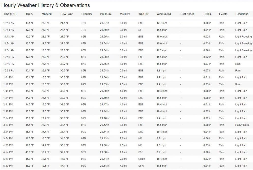
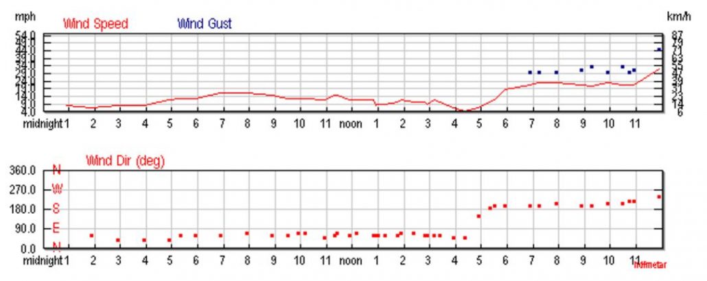
Screen captures of weather statistics on February 7, 2017 (Source: wunderground.com). Note dominant wind direction from ENE, as well as high humidity, during morning and early afternoon, when incident took place.
Calls by FracTracker for clarification from the New York State DEC’s Division of Air Resources have gone unanswered. The only station at which the DEC monitors methane is located more than 275 miles away to the southeast, in the Bronx. In Erie County, where the incident took place, there are only four permanent ambient air pollution monitoring stations. These include stations in:
“PM” refers to particulate matter diameter. PM5, for example, denotes particulate matter 5 microns in diameter, and smaller.
The East Aurora and Elma fire departments lack the appropriate air quality detection instruments to make their own judgements on the explosive nature of these gas plumes. Instead, small towns rely on the expertise of National Fuel to arrive on the scene after a call has been made, so that National Fuel can take measurements and then respond to the community. Some residents waited over three hours for an assessment, but by this time the plume had drifted away two hours ago.
National Fuel, however, has not disclosed any of the air quality data measurements they made on February 7th when they responded to this complicated incident. Ms. Marmion and others still want to know what levels of methane were measured in the communities involved in this incident, or the specific quantity of gas that entered the air that day.
While National Fuel did not notify the residents or the school district administration in advance of the scheduled “blowdown,” their Government Affairs Representative indicated that in the future, town governments, community leaders, and the local fire companies would be alerted to the upcoming releases and maintenance work. Nonetheless, weeks after the odor incident, National Fuel has neither contacted the local community leaders, nor local law enforcement, to provide complete and detailed answers as to what actually happened on February 7th.
By Karen Edelstein, Eastern Program Coordinator, FracTracker Alliance. Special thanks to East Aurora resident Jennifer Marmion, for her insights and comments.
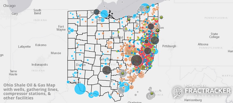
Over the last few months we’ve been busy working on some updates to our Ohio Oil & Gas Map. Check out what we’ve added recently and explore the map below!
We now have the locations of eight of the credible natural gas power plants proposed in Ohio, along with the jobs they cite during construction and operations. We also now have a complete inventory of 118 existing power plants, including 25 natural gas facilities. Together, these plants would produce 7,660 megawatts, around 957 per facility.
Six of these plants are either in the heart of Ohio’s Utica Shale or within several miles of the 1,200+ mile Appalachia-to-Texas (ATEX) pipeline. ATEX was installed to transport 190,000 barrels per day (BPD) of natural gas liquids (NGLs) from the Marcellus and Utica region to the Texas and Louisiana Gulf Goast refinery corridor. The 360 mile segment of this pipeline that runs from Pennsylvania to south central Jackson County, Indiana is also now shown on the Ohio Oil & Gas Map.
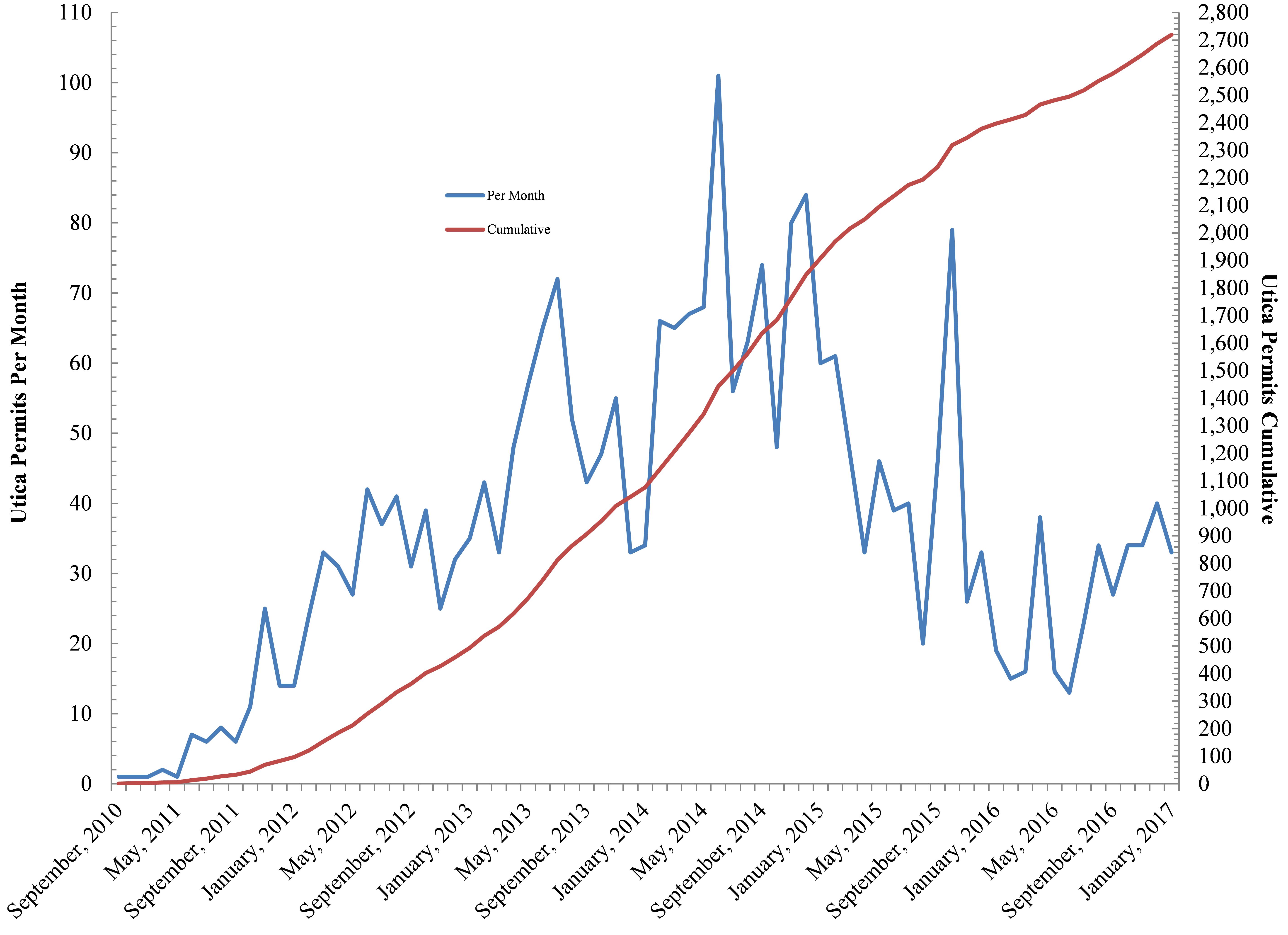
Figure 1. Cumulative and monthly hydraulic fracturing well permits in Ohio’s Utica Shale
While many shale plays across the United States are experiencing a period of contraction (with low gas prices often cited as the primary reason), drilling activity in Ohio’s Utica Shale has been experiencing a slow and steady expansion. The region has seen more than 2,700 permitted wells as of the end of January 2017. Incidentally, roughly 59% of these wells are producing either oil or gas as of Q3-2016. For more information on that subject, explore our production map.
The permitting trajectory hit a low of 13-16 permits per month between February and January of 2016. Since the presidential election in November, however, permitting rates have more than doubled (Figure 1).
Ohio sits on the western edge of both the Utica and Marcellus Shale formations, but conditions are such that the Marcellus Shale is all but being ignored in Ohio. Explore our updated map of OH drilling activity and related facilities below:
View map fullscreen | How FracTracker maps work
The map above is made up of various datasets, from the location of permits to compressor stations. These “map layers” make up the legend. Below we describe each layer on the map, as well as the data source and date range.
Horizontal Marcellus Permits, Laterals
There have been 40+ permits issued for horizontal wells in Ohio’s Marcellus Shale.
Source: Ohio Department of Natural Resources
Date Range: December 2009 – Present
Horizontal Utica Permits
An aggregate of ODNR’s monthly cumulative Utica and Marcellus permits as well as a more detailed weekly Risk Based Data Management System (RBDMS) Microsoft Access inventory. At the present time Ohio is home to 2,160+ permitted Utica Wells with the wells broken out by status. Additionally this layer contains depth, water usage, sand usage, HCl, and Gelling Agent percentage for 249 wells based on data provided to FracFocus. Finally, we have incorporated production in various units from individual industry press releases and the ODNR annual report.
Source: Ohio Department of Natural Resources
Date Range: December 2009 – Present
Horizontal Utica Permits actual and straight line laterals
An aggregate of ODNR’s monthly cumulative Utica and Marcellus permits as well as a more detailed weekly Risk Based Data Management System (RBDMS) Microsoft Access inventory. At the present time we have straight line laterals for all drilled, drilling, and producing wells as well as actual PLAT laterals for 341 of the wells.
Source: Ohio Department of Natural Resources
Date Range: December 2009 – Present
High Volume Hydraulic Fracturing Gathering Lines
All gathering lines servicing Ohio’s inventory of High Volume Hydraulic Fracturing (HVHF) wells.
Source: Herbert Hoover Foundation grant
Date Range: December 2009 – 2015
High Volume Hydraulic Fracturing Well Pads
The well-pads of all Ohio’s drilled or producing High Volume Hydraulic Fracturing (HVHF) wells.
Source: Herbert Hoover Foundation grant
Date Range: December 2009 – 2015
High Volume Hydraulic Fracturing Well Pad’s Limits Of Disturbance (LOD)
Limits Of Disturbance (LOD) for all Ohio’s drilled or producing High Volume Hydraulic Fracturing (HVHF) well-pads.
Source: Herbert Hoover Foundation grant
Date Range: December 2009 – 2015
Compressor Stations and Cracking Facilities
Boundaries of several confirmed High Volume Hydraulic Fracturing (HVHF) servicing cracking and compressor station facilities.
Source: Herbert Hoover Foundation grant
Date Range: December 2009 – 2015
Ohio Active Class II Injection Wells
This data speaks to the state’s “Active” Class II Injection wells able to accept hydraulic fracturing waste. There are 240+ Active Wells with 51 having yet to receive waste from hydraulic fracturing. For more on Ohio’s Class II Inventory in depth refer to our recent Ohio Fracking Waste Transport & Disposal Network article.
Source: Ohio Department of Natural Resources
Date Range: Historical to October, 2015
Earthquakes of >2.0 Magnitude
This data speaks to the state’s 258 earthquakes with current updates from the Ohio Seismic Network and historical quakes – all >2.0 magnitude. These data come from the department’s inventory. Additionally, we present Ohio earthquakes with <2.0 magnitude courtesy of Environment Canada’s Search the Earthquake Database platform.
Source: Ohio Department of Natural Resources, Division of Geological Survey, The Ohio Seismic Network
Date Range: Historical to Present
![]()
216 Franklin St, Suite 400, Johnstown, PA 15901
Phone: +1 (717) 303-0403 | info@fractracker.org
FracTracker Alliance is a 501(c)3 non-profit: Tax identification number: 80-0844297


