Pipeline Incidents Updated and Analyzed

Pipeline spill in Mayflower, AR on March 29, 2013. Photo by US EPA via Wikipedia.
The debate over the Keystone XL pipeline expansion project has grabbed a lot of headlines, but it is just one of several proposed major pipeline projects in the United States. As much of the discussion revolves around potential impacts of the pipeline system, a review of known incidents is relevant to the discussion.
A year ago, the FracTracker Alliance calculated that there was an average of 1.6 pipeline incidents per day in the United Sates. That figure remains accurate, with 2,452 recorded incidents between January 1, 2010 and March 3, 2014, a span of 1,522 days.
The Pipeline and Hazardous Materials Safety Administration (PHMSA) classifies the incidents into three categories:
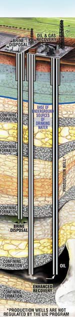
- Gas transmission and gathering: Gathering lines take natural gas from the wells to midstream infrastructure. Transmission lines transport natural gas from the regions in which it is produced to other locations, often thousands of miles away. Since 2010, there have been 486 incidents on these types of lines, resulting in 10 fatalities, 71 injuries, and $620 million in property damage.
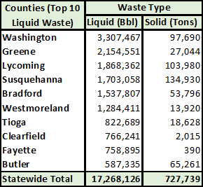
- Oil and hazardous liquid: This includes all materials overseen by PHMSA other than natural gas, predominantly crude and refined petroleum products. Liquified natural gas is included in this category. There were 1,511 incidents during the reporting period for these pipelines, causing 6 deaths and 15 injuries, and $1.8 billion in property damage.
- Gas distribution: These pipelines are used by utilities to get natural gas to consumers. In just over 40 months, there were 455 incidents, resulting in 42 people getting killed, 183 reported injuries, and $86 million in property damage.
Curiously, while incidents on distribution lines accounted for 72 percent of fatalities and 67 percent of all injuries, the property damage in these cases were only responsible for just over 3 percent of $2.5 billion in total property damage from pipeline spills since 2010. A reasonable hypothesis accounting for the deaths and injuries is that distribution lines are much more common in densely populated areas than are the other types of pipelines; an incident that might be fatal in an urban area might go unnoticed for days in more remote locations, for example. However, as the built environment is also much more densely located in urban areas, it does seem surprising that reported property damage isn’t closer to being in line with physical impacts on humans.
How accurate are the data?
In the wake of the events of September 11, 2001, governmental agency data suddenly became much more opaque. In terms of pipelines, public access to the pipeline data that had been mapped to that point was removed. It was later restored, with limitations. As it stands now, most pipeline data in the United States, including the link to the pipeline proposal map above, are intentionally generalized to the point where pipelines might not even be rendered in the appropriate township, let alone street.
There are some exceptions, though. If you would like to know where pipelines are in US waters in the Gulf of Mexcio, for example, the Bureau of Ocean Energy Management makes that data not only accessible to view, but available for download on data.gov, a site dedicated to data transparency. While the PHMSA will not do the same with terrestrial pipelines, the do release location data along with their incident data.
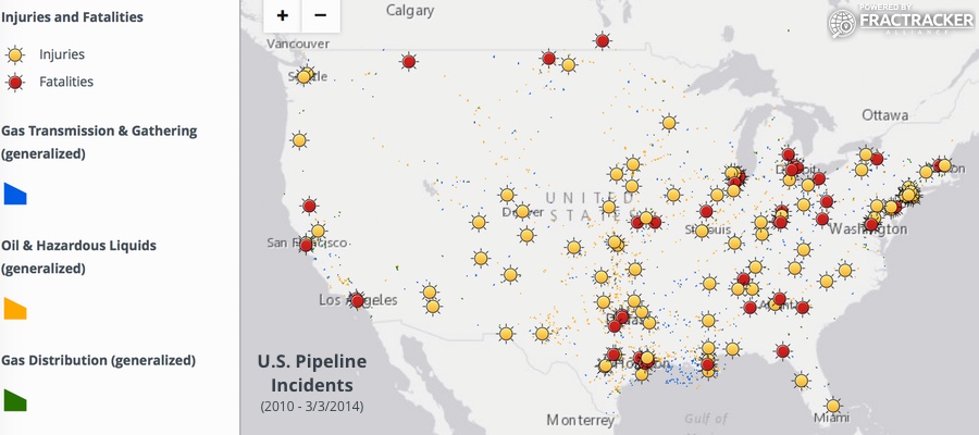
Pipeline incidents from 1/1/2010 through 3/3/2014. To access details, legend, and other map controls, please click the expanding arrows icon in the top-right corner of the map.

This fatal pipeline incident was in Allentown, PA, but was given coordinates in Greenland.
Unfortunately, we see evidence that the data are not well vetted, at least in terms of location. One of the most serious incidents in the timeframe, an explosion in Allentown, Pennsylvania that killed five people and injured three more, was given coordinates that render in the middle of Greenland. Another incident leading to fatalities was given location data that put it in Manatoba, well outside of the reach of the US agency that publishes the data. Still another incident appears to be in the Pacific Ocean, 1,300 miles west-southwest of Mexico. There are many more examples as well, but the majority of incidents seem to be reasonably well located.
Fuzzy data: are national security concerns justified?
Anyone who watches the news on a regular basis knows that there are people out there who mean others harm. However, a closer look at the incident data shows that pipelines are not a common means of accomplishing such an end.
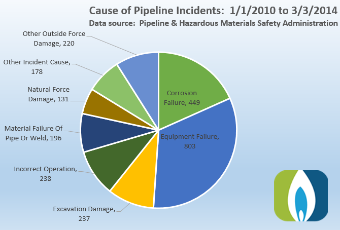
Causes of pipeline incidents from 1/1/10 to 3/3/14, with counts.
For each category showing causation, there are numerous subcategories. While we don’t need to look into all of those here, it is worth pointing out that there is a subcategory of, “other outside force damage” that is designated as, “intentional damage.” Of the 2,452 total incidents, nine incidents fall into this subcategory. These subcategories are further broken down, and while there is an option to express that the incident is a result of terrorism, none have been designated that way in this dataset . Five of the nine incidents are listed as acts of vandalism, however. To be thorough, and because it provides a fascinating insight into work in the field, let’s take a look at the narrative description for each incident that are labeled as intentional in origin:
- Approximately 2 bbls of crude oil were released when an unknown person(s) removed the threaded pressure warning device on the scraper trap’s closure door. As a result of the absence of the 1/2 inch pressure warning device crude oil was able to flow from the open port upon start up of the pipeline and pressurization of the scraper trap. Once this was discovered the 1/2 inch pressure warning device was properly put back into the scaper trap.
- Aboveground piping intentionally shot by unknown party. Installed stoppall on line at 176+73 (7 146′) upstream of damaged aboveground piping. Cut and capped pipeline.
- Friday october 18th at approximately 6:00 p.m. we were notified of a gas line break at Kayenta Mobile Home Park. The Navajo Police responded to an emergency call about vandals in one of the parks alley ways kicking at meters. Upon arrival they found the broke meter riser at the mobile home park and expediently used the emergency shutdown system to remedy the situation. This immediately cut service to 118 customers in the park. [Names removed] responded to the call. we arrived on site at approximately 9:30 p.m. We located the damage and fixed the system at approximately 1:30 a.m. i called the Amerigas emergency call center and informed them that we would be restarting the system the following morning and to tell our customers they would need to be home in order to restore service. We then started the procedure of shutting every valve off to all customers before restarting the system. We started the system back up at 9:30a.m. 10/19/2013. Once the system was up to full pressure and all systems were normal we began putting customers back into service. The completion of re-establishing service to all customers on the system was completed on 10/23/2013.
- A service tech was called at 1:15 am Sunday morning to respond to the Marlboro Fire Department at an apparent explosion and house fire. The tech arrived and called for additional resources. He then began to check for migrating gas in the surrounding buildings along the service to the house and in the street. no gas readings were detected. The distribution and service on call personnel arrived and began calling in additional company resources to assist in the response effort and controlling the incident. A distribution crew was called in to shut off and cut the service. Additional service techs were called in to assist in checking the surrounding buildings and in the streets at catch basins and manholes around the entire block. Gas supply personnel were called in and dispatched to take odorant samples in the houses directly across from 15 Grant Ct. that had active gas service. Gas survey crews were called in to survey Grant St. and the two parallel streets McEnelly St. and Washington Ct. along with the portion of Washington st. in between these streets. The meter and meter bar assembly were taken by the investigators as evidence. The service was pressure tested to the riser which was witnessed by a representative of the DPI. The service was cut off at the main. After the investigators completed gathering evidence at the scene they gave permission to begin cleaning up the site. There was a tenant home at the time of the explosion who was conscious and walking around when the fire department arrived. He was taken to the hospital and reports are that he sustained 2nd and 3rd degree burns on portions of his body.
- On Friday, September 7, 2012 PSE&G responded to a gas emergency call involving a gas ignition. The initial call came in from the Orange Fire Department at 17:09 as a house fire at 272 Reock Ave Orange; the fire chief stated gas was not involved and the fire was caused by squatters. Subsequent investigation of the incident revealed that the fire was caused when one of the squatters lit a match which ignited leaking gas originating from gas piping removed from the head of an inside meter set. The gas meter inlet valve and associated piping were all removed by an unknown person on an unknown date prior to the fire. An appliance service tech responded and shut the gas off at the curb at 17:40 on September 7 2012. A street crew was dispatched and the gas service to 272 reock ave was cut at the curb at 19:00. Two people (names unknown) squatters were injured one by the fire one was injured jumping out a window to escape the fire. The home in question was vacated by the owner and the injured parties were trespassing on the property at the time of the incident. PSE&G has been unable to confirm any information on the status of their injuries due to patient confidentiality laws.
- The homeowner tampered with company piping by removing 3/4″ steel end cap with a 3/4″ steel nipple on the tee was removed which caused the gas leak in the basement and resulted in a flash fire. The most likely source of ignition was the water heater. The homeowner died in the incident.
- A structure fire involved an unoccupied hardware store and a small commercial 12-meter manifold. There were no meters on the manifold and no customers lost service. The heat from the structure fire melted a regulator on the manifold which in turn released gas and contributed to the fire. The cause is officially undetermined; however according to the fire department the cause appears to be arson with the fire starting in the back of the building and not from PG&E facilities. PG&E was notified of this incident by the fire department at 1802 hours. The gas service representative arrived on scene at 1830 hours. The fire department stopped the flow of gas by closing the service valve and the fire was extinguished at approximately 1900 hours. this incident was determined to be reportable due to damages to the building exceeding $50,000. There were no fatalities and no injuries as a result of this incident. Local news media was on-site but no major media was present.
- A house explosion and fire occurred at approximately 0208 hours on 2/7/10. The fire department called at PG&E at 0213 hours. PG&E personnel arrived at 0245 hours. The fire department had shut off the service valve and removed the meter before PG&E arrived. The house was unoccupied at the time of the explosion. The gas service account was active and the gas service was on (contrary to initial report). The cause of the explosion is undetermined at the time of this report but the fire department has indicated the cause appears to be arson. After the explosion, PG&E performed a leak survey of the service the services on both sides of this address and the gas main in the front of all three of these addresses. No indication of gas was found. PG&E also performed bar hole tests over the service at 3944 17th Avenue and found no indication of gas. The gas service was cut off at the main and will be re-connected when the customer is ready for service.
- On Monday, January 25, 2010 at approximately 2:30pm a single-family home at 2022 west 63rd Street Cleveland OH (Cuyahoga County) was involved in an explosion/fire. The gas service line was shut-off at approximately 4:30pm. A leak survey of the main lines and service lines on W. 83rd between Madison and Lorain revealed no indications of gas near the structure. A service leak at 2131 West 83rd Street was detected during the leak survey. This service line was replaced upon discovery. On Tuesday, January 26th, 2010 the service line at 2022 W. 83rd was air tested at operating pressure with no pressure loss. An odor test was conducted at 2028 West 83rd Street. The results of this odor test revealed odor levels well within dot compliance levels. Our investigation revealed an odor complaint at this residence on January 18th. Dominion personnel responded to the call and met with the Cleveland Fire Department. Dominion found the meter disconnected and the meter shut-off valve in the half open position. The shut-off valve was closed by the Dominion technician and secured with a locking device. The technician placed a 3/4 inch plug in the open end of the valve. The technician also attempted to close the curb-slop valve but could not. The service line was then bar hole tested utilizing a combustible gas indicator from the street to the structure. As a result, no leakage was discovered. A second attempt to close the curb box valve on January 19th ended when blockage was discovered in the valve box. The valve box was in the process of being scheduled for excevatlon and shut off by a construction crew at the time of the incident. An investigation of the incident site determined the cause to be arson as approximately 6 inches of service line and the meter shut-off valve (with locking device still intact) detached from the service line were recovered inside the structure.
While several of these narratives do make it seem as if the incidents in question were deliberate, these seem to have been caused by people on the ground, not by some GIS-powered remote effort. Seven of the nine incidents were on distribution lines, which tend to occur in populated areas, where contact with gas infrastructure is in fact commonplace, and six out of those seven incidents occurred inside houses or other structures.
On the other hand, there is a real danger in not knowing where pipelines are located. 237 accidents were due to excavation activities, and 86 others were caused by boats, cars, or other vehicles unrelated to excavation activity. Better knowledge of the location of these pipelines could reduce these numbers significantly.
 The use of hydraulic fracturing for natural gas extraction has greatly increased in recent years in the Marcellus Shale. Since the beginning of this shale gas boom, water resources have been a key concern; however, many questions have yet to be answered with a comprehensive analysis. Some of these questions include:

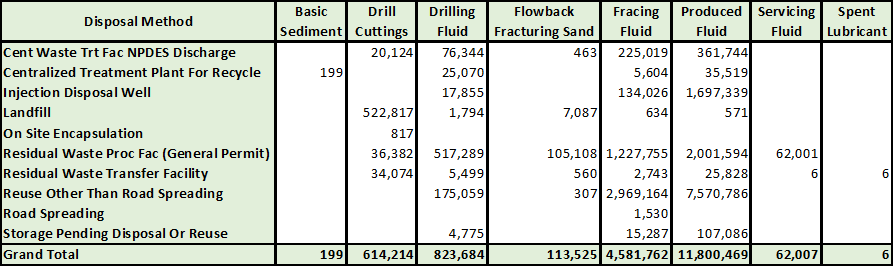
 Will recycling unconventional drilling wastewater be the solution to fresh water withdrawal impacts? Currently, it is not the goal of the industry to recycle the wastewater to potable standards, but rather to treat it for future hydraulic fracturing purposes. If the fluid immediately flowing back from the fractured well (flowback) or rising back to the surface over time (produced water) meets a certain quantity and quality criteria, it can be recycled and reused in future operations. Recycled wastewater can also be used for certain industrial and agricultural purposes if treated properly and authorized by regulators. However, if the wastewater is too contaminated (with salts, metals, radioactive materials, etc.), the amount of energy required to treat it, even for future fracturing purposes, can be too costly both in finances and in additional resources consumed.