The majority of FracTracker’s posts are generally considered articles. These may include analysis around data, embedded maps, summaries of partner collaborations, highlights of a publication or project, guest posts, etc.
By Brook Lenker, Executive Director, FracTracker Alliance
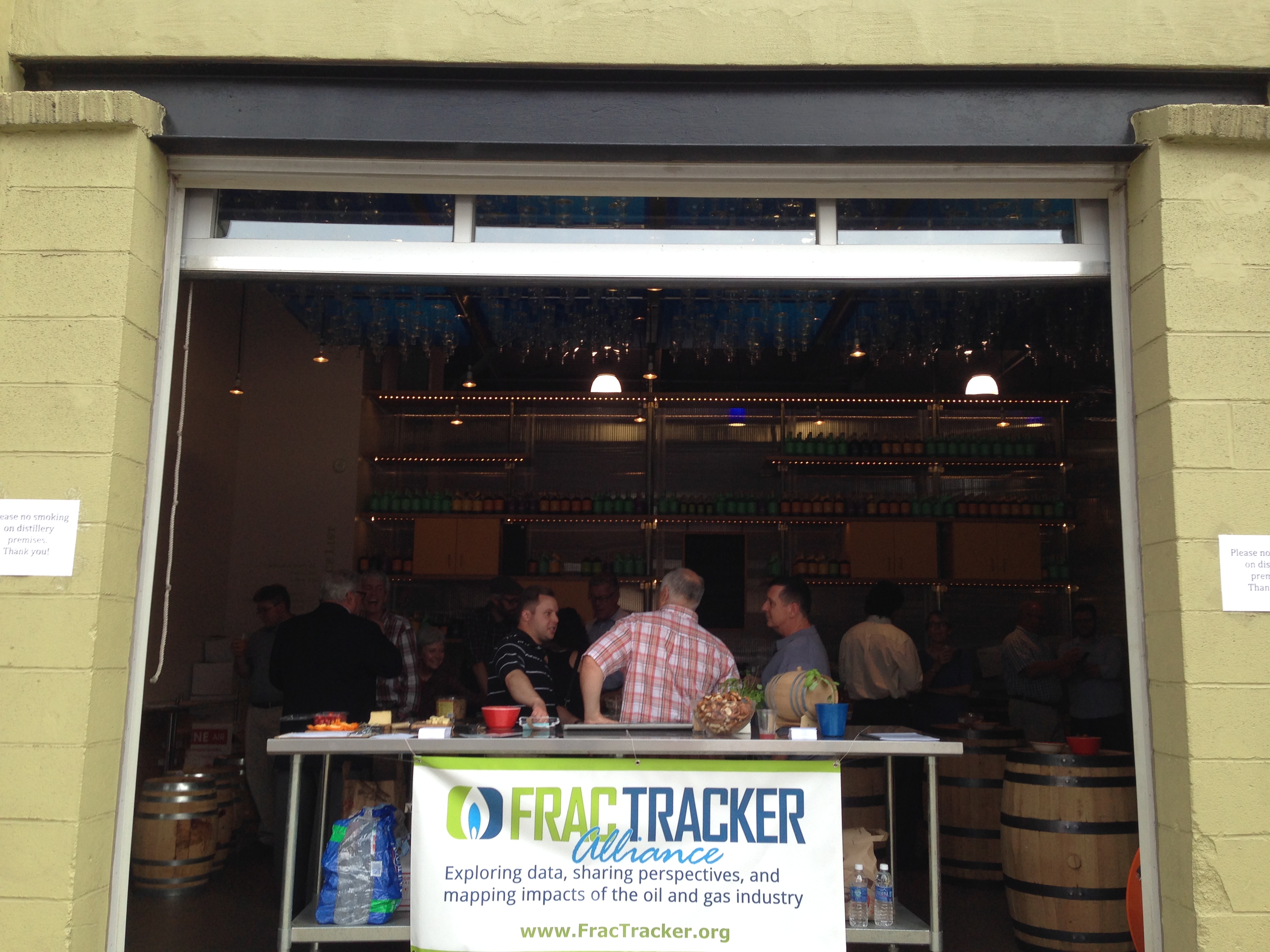
Enjoying some whiskey in Pittsburgh
It’s almost July, but just a few weeks ago, FracTracker wrapped up the last of three fundraising events. From a site in San Francisco overlooking the Pacific to a budding distillery in Pittsburgh’s Strip District, friends and colleagues came together to show their support for our work and their concern about the effects of unconventional drilling. If you were able to join us for these events – whatever the motivation, we appreciated your collective, deliberate act of kindness. Thank you!
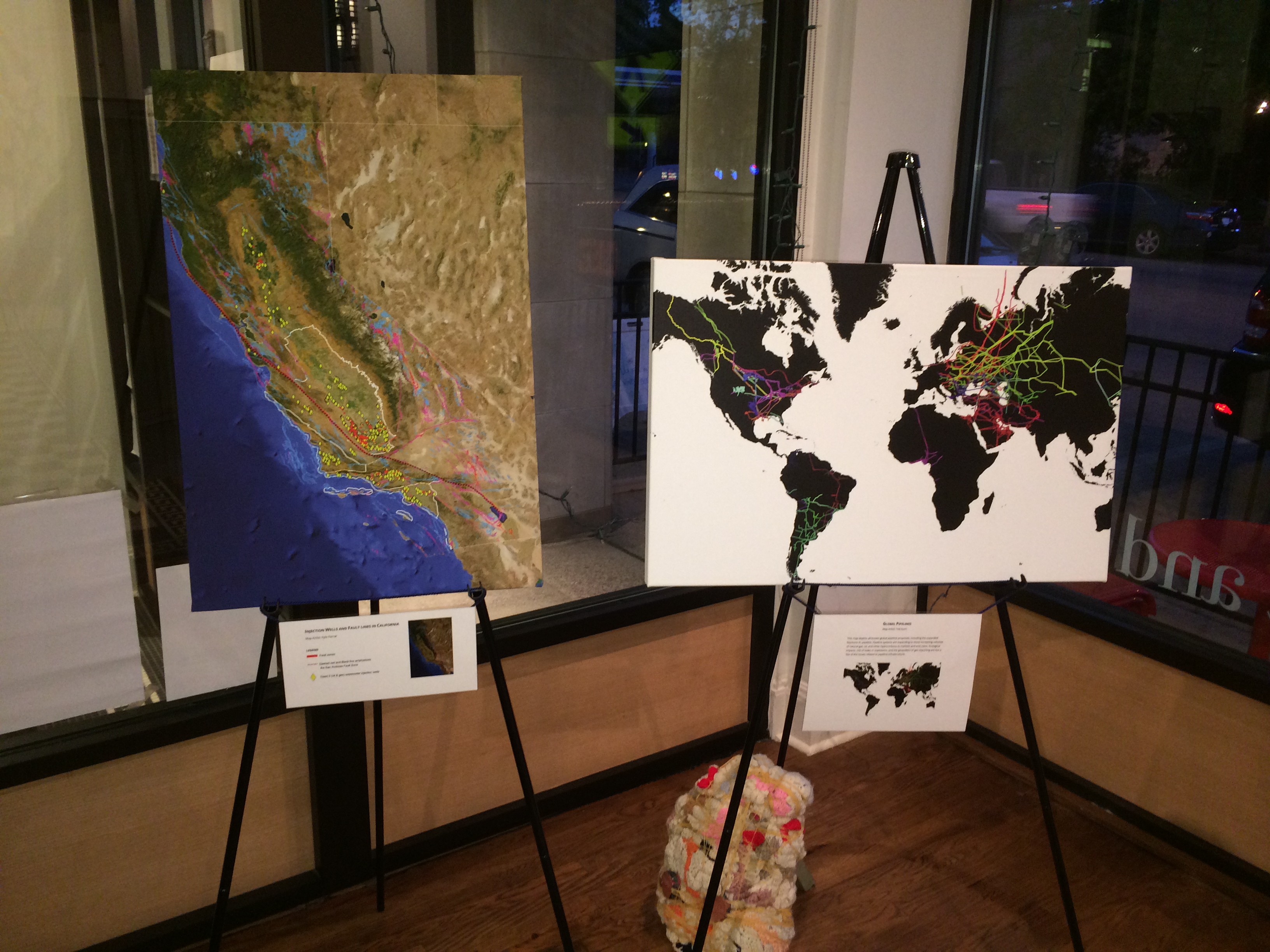
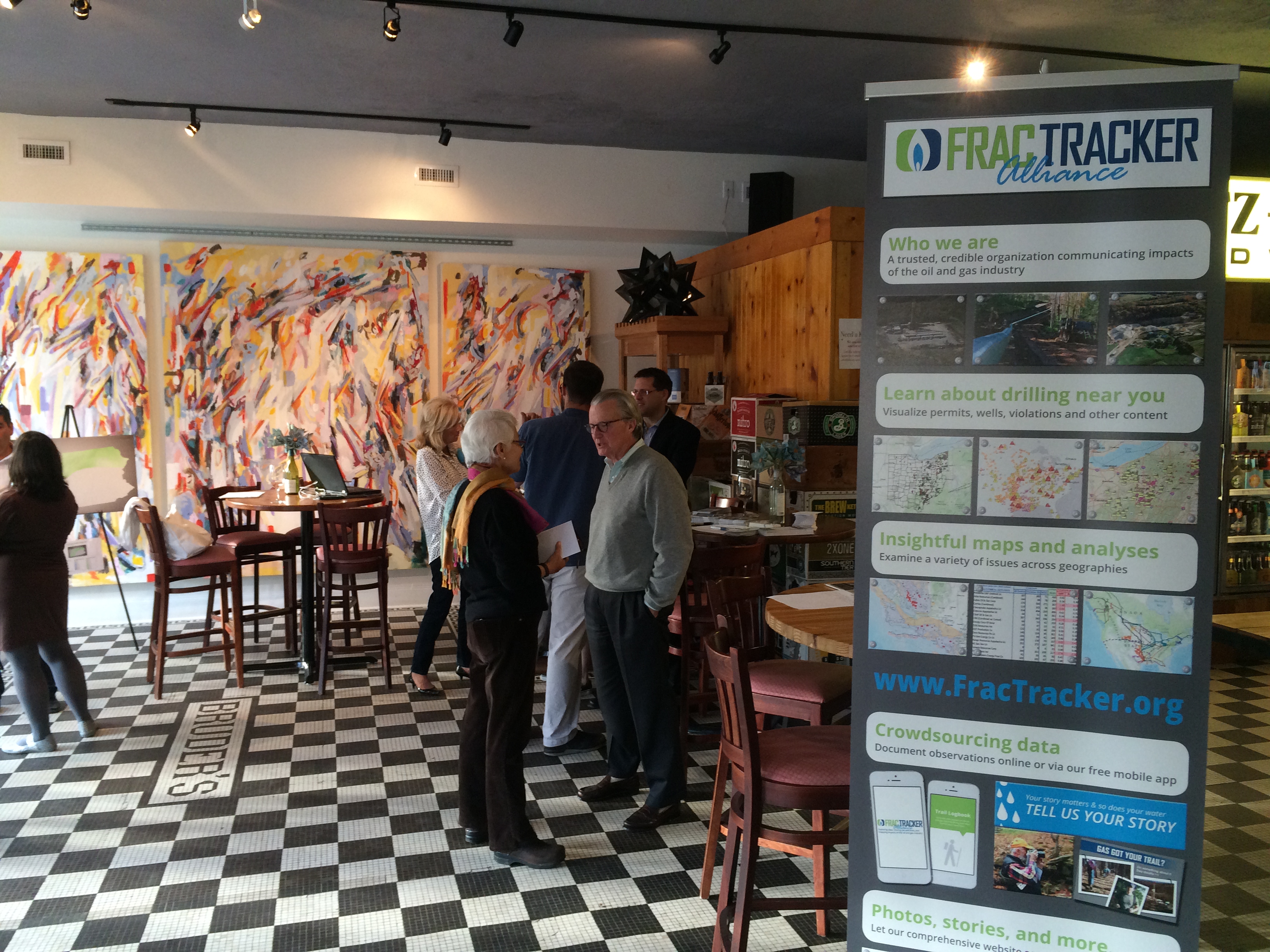
The gatherings were generally small but lots of fun – full of conversation, positive energy, and, yes, good spirits. At the Cleveland Heights event, we even had live music thanks to the jazzy guitar of Alan Brooks and at all three venues a colorful exhibit of thought-provoking, conversation-stoking maps entitled “Cartography on Canvas.” These events were our first foray into fundraisers. From the experience they’ll be improved and made even more memorable, unique, extraordinary. That’s our goal.
We aim to entice more attendees, enhance our revenue, and, most importantly, grow the network of the informed – not just informed about the activities of FracTracker but of all the groups, efforts, and learnings related to the impacts of extreme hydrocarbon extraction. Soon, another round of events – guaranteed to be mood improving, mind expanding affairs – will be rolled out. Prepare to mark your calendars, join the fun, and make your own social statement!
A special thank you goes out to FracTracker staff, interns, and board members who put in extra time and effort to help ensure the success of these initial fundraisers. Thank you, too, to our incredible door prize and auction item contributors:
https://www.fractracker.org/a5ej20sjfwe/wp-content/uploads/2014/06/IMG_6508.jpg15001500FracTracker Alliancehttps://www.fractracker.org/a5ej20sjfwe/wp-content/uploads/2025/09/2025-Wordmark-Logo.pngFracTracker Alliance2014-06-30 11:08:202020-07-21 10:42:28Putting the “Fun” in Fundraisers
By Jill Terner, PA Communications Intern, FracTracker Alliance
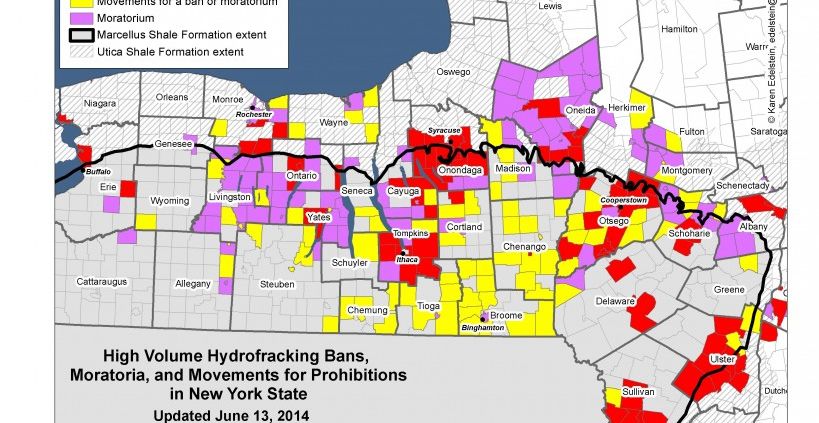
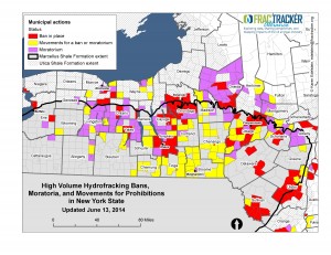
There are strong public opinions in some cases related to unconventional drilling. This map shows municipal movements in NY State against the process (06/13/2014)
In the previous two installments of this three part series, I discussed how sustainability provides a common platform for people who support and deny the use of hydraulic fracturing to extract oil and natural gas from the ground. While these opposing sides may frequently use sustainability in their rhetoric, the term has different connotations depending on which side is presented. The dynamic definition of sustainability makes it a boundary object, or a term that many people can use in shared discourse, all while defining it in different nuanced ways1. This way, the definition of sustainability alters between groups of people, and may also change over time.
First, I wrote about how pro-industry groups tend to focus primarily on the economic angle of sustainability rather than a more holistic understanding when arguing that hydraulic fracturing is the best choice for local and national communities. In my second post, I discussed how pro-environment groups see sustainability as a multifaceted entity, treating social and environmental sustainability with as much importance as economic. Here, I will focus on what can cause differences in public perceptions of hydraulic fracturing, as well as what might be done to mitigate potential confusion caused by competing definitions of sustainability.
A Few Explanations for Differing Opinions
A national survey conducted in 2013 found that by and large, people had no opinion of hydraulic fracturing. This was probably due to the fact that the majority of respondents indicated that they had heard little to nothing about hydraulic fracturing also known as unconventional drilling. Those who did identify as having an opinion either for or against drilling were split nearly evenly*. While survey participants on both sides recognized that there could be several economic benefits related to industrial presence, they also acknowledged that distribution of these benefits might not be equitable. Additionally, recognition of environmental and social threats is correlated with a negative view of industry. The stronger a respondents’ concern is about damaging environmental and social outcomes resulting from drilling activities, the more likely they were to express negative opinions about the industry2.
What is responsible for this difference of opinion? One possible explanation lies in the level of drilling activity a given community is experiencing. In areas where hydraulic fracturing is more prevalent, residents are more likely to have leased their land to drilling companies, so they are more likely to adjust their attitude to reflect their actions. They have made a significant investment by leasing their land, so they are likely to be optimistic about the payoff3.
Relatedly, the length of time that industry has been active in an area might also affect public perceptions. When industry is relatively new, many residents of nearby communities are optimistic about the economic gains that it may bring. However, alongside this optimism, residents may also express trepidation regarding what the influx of new people and wealth might do to community integrity. Over time, though, residents of areas where industry has maintained a continued presence may have adjusted to the changes brought on by industry, or have had their initial fears mitigated3, 4,5.
Geographically speaking, proximity to a major metropolitan area may also play a role in public perception of unconventional drilling. In counties where there are more metropolitan areas, there is the potential for an increase in negative social side effects. For example, an increase in violent crimes5, 6, uneven distribution of wealth generated by industry4, and loss of community character4, 6, might be offset by the fact that the influx of new workers makes up a smaller proportion of the county population than in less urbanized counties4.
On a broader geographical scale, state-by-state differences in opinion could be largely due to how prohibitive or permissive laws are regarding drilling. In states such as New York, where legislation demonstrates concern for the environment and safety, residents may be more likely to see sustainability as something more than just economic. On the other hand, in states like Pennsylvania where legislation is relatively permissive, residents may be more likely to see economic sustainability as most important due to the political climate4. This view is also known as the chicken/egg phenomenon: does the public’s opinion sway legislation, or does legislation drive public opinion? Either way, the differences across state lines remains.
What can be done to better inform public opinion?
Above, I mentioned a study where researchers found that the vast majority of survey participants held no opinion regarding unconventional drilling, largely due to lack of knowledge about it2. Therefore making unbiased information readily available and understandable to the public will allow them to make informed opinions on the subject. For example, having access to objective literature regarding unconventional drilling provides the opportunity to increase awareness and inform individuals about the practice of hydraulic fracturing and its potential impacts. In order to have the most impact we must first asses where gaps in public knowledge lie. Engaging in projects such as community based participatory research and then qualitatively assessing the results will reveal common misconceptions or knowledge gaps that need to be addressed through educational programs.
Also, most predictions regarding the unconventional drilling boom are based on a boom-and-bust cycles of past industries4. For example, they look at longitudinal studies where representative groups of residents within communities are followed over time, and they also focus on existing communities affected by industry identifying the social, environmental, and economic outcomes related to industry. This way, any comparisons drawn would be within the same industry, even if they were between two different cities.
Finally, the information gleaned from community based participatory or longitudinal research should be presented by an unbiased party and made easily available. Promoting transparency within biased institutions is equally important. While each entity uses the term “sustainability” to dynamically fit its rhetorical needs, few entities prioritize the same kinds of sustainability. Therefore, it is up to industry, environmental groups, and independent researchers alike to provide a transparent atmosphere of honest information so that individuals can decide which understanding of sustainability they would like to see informing the progress of unconventional drilling in their communities.
About the Author
Jill Terner is an MPH candidate at Columbia University’s Mailman School of Public Health and a native Pittsburgher. Interning with FracTracker in fall of 2013 has cemented Jill’s interest in combining Environmental Public Health with her passion for Social Justice. After completing her MPH in May 2015, Jill hopes to find work helping people better understand, interact with, and mitigate threats to their environment – and how their environment impacts their health.
Footnotes
* 13% did not know how much they had heard about drilling, 39% had heard nothing at all, 16% had heard “a little”, 22% had heard “some”, and 9% had heard “a lot.” Of these respondents, 58% did not know/were undecided about whether they supported drilling, 20% were opposed, and 22% were supportive2.
Sources
Star, S. L., & Griesemer, J. R. (1989). Institutional ecology, ‘translations’ and boundary objects: Amateurs and professionals in Berkeley’s museum of vertebrate zoology, 1907-39. Social Studies of Science, 19, 387-420.
Boudet, H., Carke, C., Bugden, D., Maibach, E., Roser-Renouf, C., & Leiserowitz, A. (2013). “fracking” controversy and communication: Using national survey data to understand public erceptions of hydraulic fracturing. Energy Policy, 65, 57-67.
Kriesky, J., Goldstein, B. D., Zell, K., & Beach, S. (2013). Differing opinions about natural gas drillingin two adjacent counties with different livels of drilling activity. Energy Policy, 50, 228-236.
Wynveen, B. J. (2011). A thematic analysis of local respondents’ perceptions of barnett shale energy development. Journal of Rural Social Sciences, 26(1), 8-31.
Brasier, K. J., Filteau, M. R., McLaughlin, D. K., Jacquet, J., Stedman, R. C., Kelsey, T. W., & Goetz, S. J. (2011). Residents’ perceptions of community and environmental impacts from development of natural gas in the Marcellus Shale: A comparison of Pennsylvania and New York cases. Journal of Rural Social Sciences, 26(1), 32-61.
Korfmacher, K. S., Jones, W. A., Malone, S. L., & Vinci, L. F. (2013). Public Health and High Volume Hydraulic Fracturing. New Solutions, 23(1) 13-31.
https://www.fractracker.org/a5ej20sjfwe/wp-content/uploads/2012/04/municipal_movements_against_rev06-132014_MAP-e1402678058310.jpg633819FracTracker Alliancehttps://www.fractracker.org/a5ej20sjfwe/wp-content/uploads/2025/09/2025-Wordmark-Logo.pngFracTracker Alliance2014-06-25 12:51:542020-07-21 10:42:28Public Perception of Sustainability
By Karen Edelstein, NY Program Coordinator, FracTracker Alliance
Background
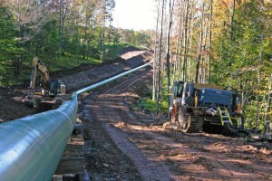
Over the past month and a half, a new pipeline controversy has been stirring in Pennsylvania. The proposed $2 billion “Central Penn Pipeline” will be built to carry shale gas throughout the country. Starting in Susquehanna County, the 178 mile pipeline will run through Lebanon and Lancaster counties to connect the existing Tennessee Pipeline in the north with the Transco Pipeline in the south.
Oklahoma-based Williams Partners, the company proposing the pipeline, says that the project would help move gas from PA to locations as far south as Georgia and Alabama, in addition to adding relief from higher energy bills. The “Atlantic Sunrise Project,” as it is formally known, would also require the construction of two new 30,000 horse-power compressor stations: “Station 605” along the northern leg of the pipeline in Susquehanna County, as well as “Station 610” on the southern part of the pipeline. The northern part of the proposed pipeline will be 30 inches in diameter and run for about 56 miles; the southern portion will be 42 inches in diameter and about 122 miles long.
According to the US Energy Information Agency (EIA), in 2008, PA had over 8,700 miles of pipeline. Since then, that figure has increased significantly as the shale plays in PA continue to be exploited. Industry maintains that pipelines are the safest method for moving gas from the well to market, and has noted that for safety concerns they have intentionally co-located 36% of the northern part of the pipeline within the rights-of-way of Transco’s or other utility’s pipelines.
Despite the sanguine view of this project by industry, residents have rallied against the pipeline since mid-April, when landowners started getting information packets in the mail about the proposal.
Pipeline Proposal Map
While the exact route of the pipeline has yet to be determined, FracTracker has adapted documents from Oklahoma-based Williams Partners Company to provide this interactive map below. The proposed pipeline is shown in red.
For a full-screen version of this map (with legend), click here.
Proposal Concerns
Public awareness and concern about the pipeline continues to build, as was evident when 1,100 residents attended an open house in Millersville, PA on June 10th hosted by Williams. For more information see this article in Lancaster Online.
The Lancaster County Conservancy has advocated moving the pipeline away from various sensitive habitats including the Tucquan Glen Nature Preserve, Shenk’s Ferry Wildflower Preserve, Fishing Creek, Kelly’s Run, and Rock Springs to preserve the wildlife and beauty of those areas. According to Williams:
The pipeline company must evaluate a number of environmental factors, including potential impacts on residents, threatened and endangered species, wetlands, water bodies, groundwater, fish, vegetation, wildlife, cultural resources, geology, soils, land use, air and noise quality… More
Despite what the website says, Williams admitted to not analyzing the pipeline route for possible sensitive habitat encroachment, and instead, they will simply follow the existing utility routes.
Williams, according to a report by WGAL Channel 8 in PA “relies on the communities affected to bring up any potential problems.” His statement was backed up when residents in a packed hearing room in Lancaster County voiced their opposition, resulting in Williams Partners now considering extending their pipeline by 2 ½ miles to get around the sensitive natural area at Tucquan Glen. An alternate route to avoid Shenk’s Ferry, however, had not been put forward.
Lancaster Farmland Trust is concerned about the plan for the pipeline to pass through several protected farms, and Lebanon County Commissioner Jo Ellen Litz has also taken a strong stand against the current proposed route. The proposed pipeline would not only go through farmlands, but it is also expected to cross the Appalachian Trail, Swatara State Park, and Lebanon Valley Rails to Trails.
Pipeline impacts are not limited to conservation and agriculture. There is increasing concern that the risks posed by large-diameter, high pressure pipelines such as this one may prevent nearby homeowners from keeping their mortgage loans or homeowner’s insurance. Future purchasers of the property may also encounter difficulty being approved for a mortgage loan or homeowner’s insurance.
While the pipeline company can purchase pipeline easements from property owners, industry can also petition the government to take the land by eminent domain from unwilling property owners. Pipeline rights-of-way acquired through eminent domain for these pipelines could potentially complicate a private property owner’s mortgage financing and homeowner’s insurance.
The final decisions about the siting of the pipeline is ultimately up to FERC, the Federal Energy Regulatory Commission.
Resources
Williams’ original maps of the pipelines can be viewed here: SOUTH | NORTH
https://www.fractracker.org/a5ej20sjfwe/wp-content/uploads/2014/06/5550c-Pipeline-Marc-1-e1403196615466.jpg200300Karen Edelsteinhttps://www.fractracker.org/a5ej20sjfwe/wp-content/uploads/2025/09/2025-Wordmark-Logo.pngKaren Edelstein2014-06-20 10:17:192020-07-21 10:42:27Central Penn Pipeline Under Debate
By Ted Auch, OH Program Coordinator, FracTracker Alliance
No matter where you live in Ohio you have probably asked yourself if crime trends will be – or have already been – affected by the shale gas boom.
To quantify the relationship between crime rates and oil and gas development, we compared 14 OH counties (that have more than 10 Utica permits) to statewide safety metrics. Ohio State Highway Patrol’s Statistical Analysis Unit provided us with the necessary crime data. From this dataset, we chose to analyze several metrics:
a. three types of arrests,
b. two types of violations and accidents, and
c. misdemeanors and suspended licenses (as proxies for changes in safety).
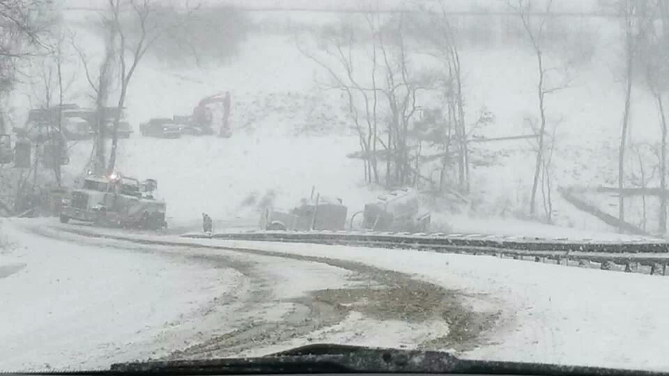
Accident involving truck carrying freshwater for fracking between Jan. 20 and 27 of 2014 during snowstorm adjacent to Seneca Lake, Noble and Guernsey Counties, OH adjacent to Antero pad off State Route 147
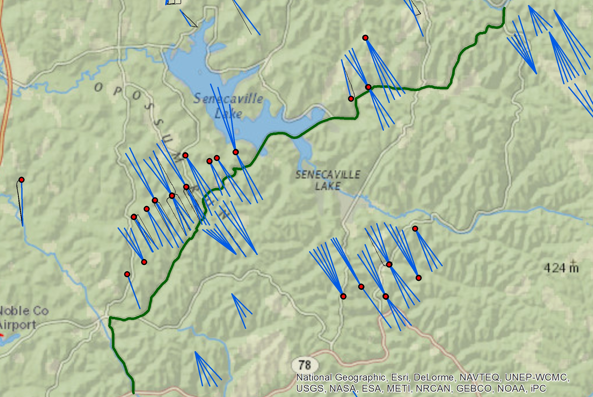
Map of Senaca Lake, OH Jan 2014 frackwater truck accident including producing or drilled Antero wells (Red Points) and laterals along with State Route 147
Crunching the Data
The data in Table 1 below are corrected for changes in population at the state level (+0.2% per year) and at the county level, with the annualized rate for the counties of interest ranging between -2.2% in Jefferson and -0.05 in Tuscarawas. We used the first four months of 2014 to determine an annualized rate for the rest of 2014. Since the first Utica permit was issued on Sept. 28, 2010, we assumed that the 2009 data would be an close measure for the ambient levels for the nine crime metrics we investigated across Ohio prior to shale gas development.
Statewide Crime Trends
Overturned frac sand trucks in Carroll County, OH May, 2014 (Courtesy of Carol McIntire, The Free Press Standard)
Commercial Vehicle Enforcements (CVE) and Crashes Investigated are the only metrics that increase by 8.9% and 6.9% per year, larger than the statewide averages of 2.8% and 6.0%. Respectively, 10 of the 14 shale gas counties have experienced rates that exceed the state average. Noble, Harrison, Columbiana, Carroll, and Monroe are experiencing annualized CVE increases that are 15-57% higher than Ohio as a whole.
Meanwhile, Crashes Investigated are increasing at a slower pace relative to the state wide average, with Carroll, Noble, and Jefferson counties experiencing >5% rate increases relative to the entire state (Table 1). There is a strong increasing linear relationship between the number of Utica permits and the average percent change in CVE and Crashes Investigated. The former accounts for a combined 66% change in the latter. From a macro perspective, the Utica counties accounted for 19.8% of all OH CVEs in 2009 prior to shale gas exploration and now account for 25.1% of all CVEs. Crashes Investigated as a percentage of state totals, however, only increased from 21.3% to 21.7%.
The other variable that is significantly and positively correlated with Utica permitting at the present time is the number of Suspended License reports, with the former explaining 22% of the average annual change in the latter since 2009.
Given that we investigated changes in nine public safety metrics we thought it would be worth categorizing the fourteen counties by state wide averages:
Significantly Less Safe (SLS) – >5 of 9 metrics increasing,
Noticeably Less Safe (NLS) – 4 metrics, and
Marginally Less Safe (MLS) – <3 metrics.
Our findings support that about half the Utica counties fall within the SLS category, with Harrison, Jefferson, Columbiana, and Trumbull experiencing higher relative rates across seven or more of the metrics investigated. Trumbell specifically has had public safety rate increases that are greater than the state in all categories but for Suspended Licenses. Guernsey and Washington counties fall within the NLS category; both are seeing elevated Resisting Arrests and CVEs relative to changes in statewide rates. Surprisingly, Carroll County, home to 404 Utica permits as of the middle of May 2014, falls within the MLS category with only two of nine metrics increasing at a rate that exceeds the state’s. However, the two metrics that are worse than the state average (Crashes Investigated (+21.4%) and CVEs (59.8%)) are increasing at a rate that is significantly higher than the other Ohio Utica counties. Additional MLS counties include Belmont, Portage, and Monroe, which are in the upper, middle, and lower third of Utica permits at the present time.
Conclusion
While correlation does not mean causation, there is a significant correlation between certain public safety metrics and Utica permitting in Ohio’s primary shale gas counties, specifically when looking at Crashes Investigated and CVEs. Additionally, many of the Ohio Utica counties are experiencing notable increases in criminal activity. Whether this trend will continue to increase in the long-term is uncertain, but the short-term trends are concerning given that these counties populations are decreasing; there is more criminal activity within a smaller population. Finally, these trends will differ based on whether or not county sheriffs and emergency responders working with the Ohio State Highway Patrol have the necessary resources and manpower to address increasing criminal activity. This issue is of concern to most southeastern Ohioans regardless of their stance on fracking. We will continue to monitor these relationships and are working to generate a map in the coming months that illustrates these trends.
Table 1. Average percent change in select public safety metrics across Ohio’s primary Utica Shale Counties relative to parallel changes across the state of Ohio between 2009 and 2014.
Percent Change Between 2009 and 2014†
Arrests
Violations
County
Felony
Resisting
OVI
Weapons
Drug
Crashes Investigated
CVE
Misdemeanor Issued
Suspended License
Noble (93, 6‡)
87.7
0
10.5
16.9
16.8
11.2
50.5
11.8
7.4
Harrison (232, 0)
22.3
0
35.8
0
34.3
10.1
34.7
67.1
33.3
Belmont (102, 2)
12.7
5.5
2.2
17.2
20.3
10.5
4.0
16.6
10.2
Jefferson (39, 1)
50.1
3.6
11.6
43.3
45.9
11.3
12.5
42.0
10.4
Columbiana (103, 0)
20.3
-3.8
6.9
28.9
27.1
7.9
17.8
25.9
10.6
Tuscarawas (16, 6)
41.2
28.9
7.0
0
0.8
7.6
12.0
61.4
3.6
Washington (10, 13)
10.1
52.7
-2.7
47.3
19.8
8.3
4.6
19.2
2.6
Stark (13, 17)
7.3
9.4
0.3
46.4
7.2
6.7
2.6
11.1
-0.5
Trumbull (15, 20)
32.9
18.9
8.6
42.9
42.1
9.3
11.5
41.1
9.4
Mahoning (30, 10)
21.4
20.7
3.6
81.4
31.8
6.0
8.5
27.7
10.2
Portage (15, 19)
80.7
4.5
4.1
85.0
40.3
3.5
1.6
15.5
7.6
Guernsey (99, 5)
22.8
32.9
8.1
14.7
10.4
2.7
11.0
10.8
7.6
Carroll (404, 4)
0
0
-20.2
0
-29.1
21.4
59.8
-30.2
3.8
Monroe (80, 0)
0
0
-4.1
0
0
97.4
50.8
20.4
27.0
County
16.5
4.3
3.5
10.3
17.6
6.9
8.9
17.8
5.8
State
17.4
6.7
7.3
16.5
23.6
6.0
2.8
24.5
10.5
% of State 2009
14.0
17.6
19.3
18.7
16.1
21.3
19.8
17.8
18.4
% of State 2014
12.9
15.2
16.7
16.8
14.0
21.7
25.1
13.1
14.5
† 2014 annualized using the first 4 months of the year.
‡ Number of Permitted Utica wells and Class II Salt Water Disposal (SWD) wells as of May, 2014
https://www.fractracker.org/a5ej20sjfwe/wp-content/uploads/2014/06/Sand-truck-rollover-for-Fractracker.jpg255432Ted Auch, PhDhttps://www.fractracker.org/a5ej20sjfwe/wp-content/uploads/2025/09/2025-Wordmark-Logo.pngTed Auch, PhD2014-06-09 14:26:222020-07-21 10:42:27Crime and the Utica Shale
By Andrew Donakowski, Northeastern Illinois University
Land cover data can play an important role in spatial analysis; satellite or aerial imagery can effectively demonstrate the extent and make-up of land cover characteristics for large areas of land. For fracking analysis, this can be used to explore important spatial relationships between fracking infrastructure and the area and/or ecosystems surrounding them. Working with FracTracker, I have compiled data concerning land cover classifications and geologic rock areas to examine areas that may be particularly vulnerable to unconventional drilling – e.g. fracking. After computing the makeup of land cover type for each geologic area, I then mapped locations of known fracking wells for further analysis. This is part of FracTracker’s ongoing interest in understanding changes in ecosystem services and plant/soil productivity associated with well pads, pipelines, retention ponds, etc.
Developed
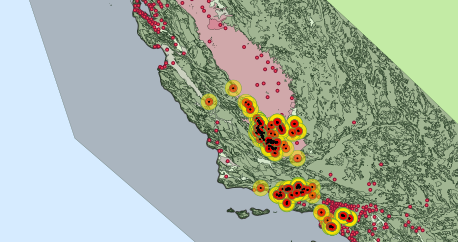
First, by looking at the Developed areas (below), we can see that, for the most part, hydraulic fracturing is occurring relatively far from large population areas. (That is to say, on this map we can see that these types of wells are not found as often in areas where population density is high (<20 people per square mile) or a Developed land cover classification is predominate as they are in areas with a lower Develop land cover percentage). However, we can also see that there is quite a large cluster of fracking wells in the southern portion of the state, and many cities fall within 5 or 10 mi of some wells. While there may not be an immediate danger to cities that fall within this radius, we can see that some areas of the state may be more likely to encounter the effects of fracking and its associated infrastructure than others.
Forested
Next, the map depicting Forested land cover areas is, in my opinion, the most aesthetically groovy of the land cover maps; the variations in forested areas throughout the state provide a cool image. By looking at this data, we can see that much of California’s forested land lies in the northern part of the state, while most fracking wells are located in the south and central parts of the state.
Cultivated
To me, the most interesting map is the one below showing the location of fracking wells in relation to Cultivated lands (which includes pasture areas and cropland). What is interesting to note is the fertile Central Valley, where a high percentage of land is covered with agriculture and pasture lands (Note: The Central Valley accounts for 1% of US farmland but 25% of all production by value). Notably, it is also where many fracking wells are concentrated. When one stops to think about this, it makes sense: Farmers and rural landowners are often approached with proposals to allow drilling and other non-farming activities on their land. Yet, it also raises a potential area for concern: A lot of crops grown in this area are shipped across the country to feed a significant number of people. When we consider the uncertainties of fracking on surrounding areas, we must also consider what effects fracking could have beyond the immediate area and think about how fracking could affect what is produced in that area (in this case, it is something as important as our food supply.)
The Usefulness of Maps
Finally, as previously mentioned, mapping the extent of these land coverage can be useful for future analysis. Knowing now the areas of relatively large concentrations of forested, herbaceous, and wetland (which can be highly sensitive to ecological intrusions) areas can be good to know down the line to see if those areas are retreating or if the overall coverage is diminishing. Additionally, by allowing individuals to visualize spatial relationships between fracking areas and land coverage, we can make connections and begin to more closely examine areas that may be problematic. The next step will be: a) parsing forest cover into as many of the six major North American forest types and hopefully stand age, b) wetland type, and c) crop and/or pasture species. All of this will allow us to better quantify the inherent ecosystem services and CO2 capture/storage potential at risk in California and elsewhere with the expansion of the fracking industry. As an example of the importance of the intersection between forest cover and the fracking industry we recently conducted an analysis of frac sand mining polygons in Western Wisconsin and found that 45.8% of Trempealeau County acreage is in agriculture while only 1.8% of producing frac sand mine polygons were in agriculture prior to mining with the remaining acreage forested prior to mining which buttresses our anecdotal evidence that the frac sand mining industry is picking off forested bluffs and slopes throughout the northern extent of the St. Peter Sandstone formation.
A Quick Note on the Data
Datasets for this project were obtained from a few different sources. First, land cover data were downloaded from the National Land cover Classification Database (NLCD) from the Multi-Resolution Land Character Consortium. Geologic data were taken from the United States Geologic Survey (USGS) and their Mineral Resources On-Line Spatial Data. Lastly, locations of fracking wells were taken from the FracTracker data portal, which, in turn, were taken from SkyTruth’s database. Once the datasets were obtained, values from the NLCD data were reclassified to highlight land-coverage types-of-interest using the Raster Calculator tool in ArcMap 10.2.1. Then, shapefiles from the USGS were overlaid on top of the reclassified raster image, and ArcMaps’s Tabulate Area tool was used to determine the extent of land coverage within each geologic rock classification area. Known fracking wells downloaded from FracTracker.org were added to the map for comparative analysis.
About the Author
Andrew Donakowski is currently studying Geography & Environmental Studies, with a focus on Geographic Information Systems (GIS), at Northeastern Illinois University (NEIU) in Chicago, Ill. These maps were created in conjunction with FracTracker’s Ted Auch and NEIU’s Caleb Gallemore as part of a service-learning project conducted during the spring of 2014 aimed at addressing real-world issues beyond the classroom.
https://www.fractracker.org/a5ej20sjfwe/wp-content/uploads/2014/05/CA-Land-Use-e1426083845893.png242458FracTracker Alliancehttps://www.fractracker.org/a5ej20sjfwe/wp-content/uploads/2025/09/2025-Wordmark-Logo.pngFracTracker Alliance2014-05-29 12:11:422020-07-21 10:42:27Fracturing wells and land cover in California
Like most states, the data from the Pennsylvania Department of Environmental Protection do not explicitly tell you which wells have been hydraulically fractured. They do, however, designate some wells as unconventional, a definition based largely on the depth of the target formation:
An unconventional gas well is a well that is drilled into an Unconventional formation, which is defined as a geologic shale formation below the base of the Elk Sandstone or its geologic equivalent where natural gas generally cannot be produced except by horizontal or vertical well bores stimulated by hydraulic fracturing.
Naturally occurring karst in Cumberland County, PA. Photo by Randy Conger, via USGS.
While Pennsylvania has been producing oil and gas since before the Civil War, the arrival of unconventional techniques has brought greater media scrutiny, and at length, tougher regulations for Marcellus Shale and other deep wells. We know, however, that some companies are increasingly looking at using the combination of horizontal drilling and hydraulic fracturing in much shallower formations, which could be of greater concern to those reliant upon well water than wells drilled into deeper unconventional formations, such as the Marcellus Shale. The chance of methane or fluid migration through karst or other natural fissures in the underground rock formations increase as the distance between the hydraulic fracturing activity and groundwater sources decrease, but the new standards for unconventional wells in the state don’t apply.
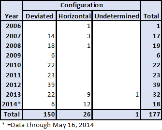
The following chart summarizes data for wells through May 16, 2014 that are not drilled vertically, but that are considered to be conventional, based on depth:
These wells are listed as conventional, but are not drilled vertically.
Note that there have already been more horizontal wells in this group drilled in 2014 than any previous year, showing that the trend is increasing sharply.
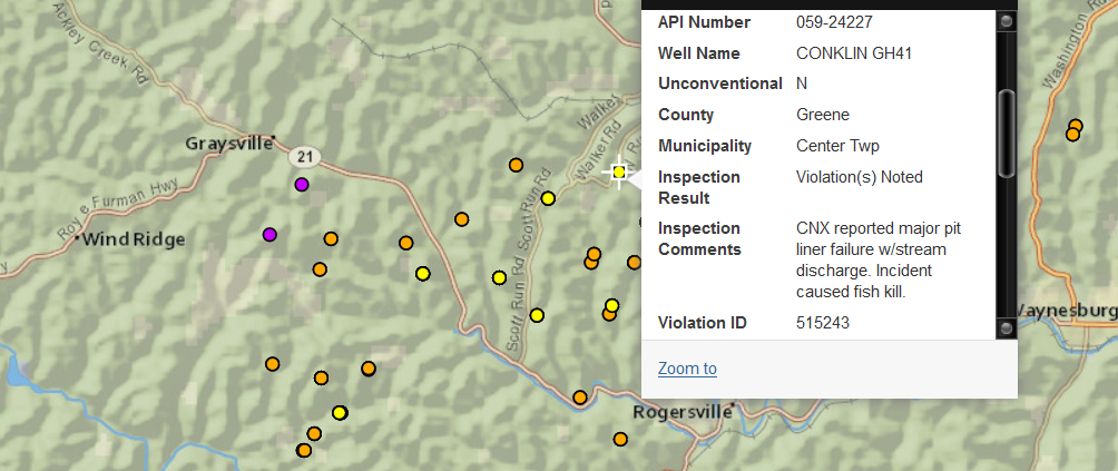
Of the 26 horizontal wells, 12 are considered oil wells, five are gas wells, five are storage wells, three are combination oil and gas, and one is an injection well. These 177 wells have been issued a total of 97 violations, which is a violation per well ratio of 62 percent. 429 permits in have been issued in Pennsylvania to date for non-vertical wells classified as conventional. Greene county has the largest number of horizontal conventional wells, with eight, followed by Bradford (5) and Butler (4) counties.
We can also take a look at this data in a map view:
Conventional, non-vertical wells in Pennsylvania. Please click the expanding arrows icon at the top-right corner to access the legend and other map controls. Please zoom in to access data for each location.
https://www.fractracker.org/a5ej20sjfwe/wp-content/uploads/2014/05/PA_CNV_BlogFeature.png5151004Matt Kelso, BAhttps://www.fractracker.org/a5ej20sjfwe/wp-content/uploads/2025/09/2025-Wordmark-Logo.pngMatt Kelso, BA2014-05-19 16:10:222020-07-21 10:42:26Conventional, Non-Vertical Wells in PA
By Samantha Malone, MPH, CPH – Manager of Science and Communications, FracTracker Alliance
The population most at risk from accidents and incidents near unconventional drilling operations are the drillers and contractors within the industry. While that statement may seem quite obvious, let’s explore some of the numbers behind how often these workers are in harm’s way and why.
O&G Risks
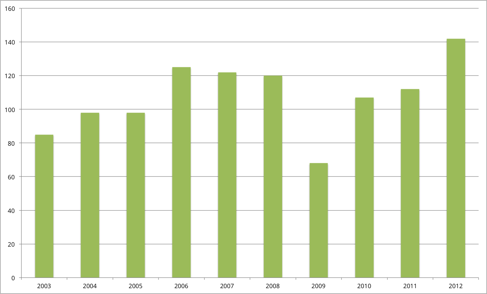
Fig. 1. Number of oil and gas worker fatalities over time Data Source: U.S. Bureau of Labor Statistics, U.S. Department of Labor, 2014
Drilling operations, whether conventional or unconventional (aka fracking), run 24 hours a day, 7 days a week. Workers may be on site for several hours or even days at a time. Simply the amount of time spent on the job inherently increases one’s chances of health and safety concerns. Working in the extraction field is traditionally risky business. In 2012, mining, quarrying, and oil and gas extraction jobs experienced an overall 15.9 deaths for every 100,000 workers, the second highest rate among American businesses. (Only Agriculture, forestry, fishing and hunting jobs had a higher rate.)
According to the Quarterly Census of Employment and Wages of the U.S. Bureau of Labor Statistics, the oil and gas industry employed 188,003 workers in 2012 in the U.S., a jump from 120,328 in 2003. Preliminary data indicate that the upward employment trend continued in 2013. However, between 2003 and 2012, a total of 1,077 oil and gas extraction workers were killed on the job (Fig. 1).
Causes of Injuries and Fatalities in Oil and Gas Field
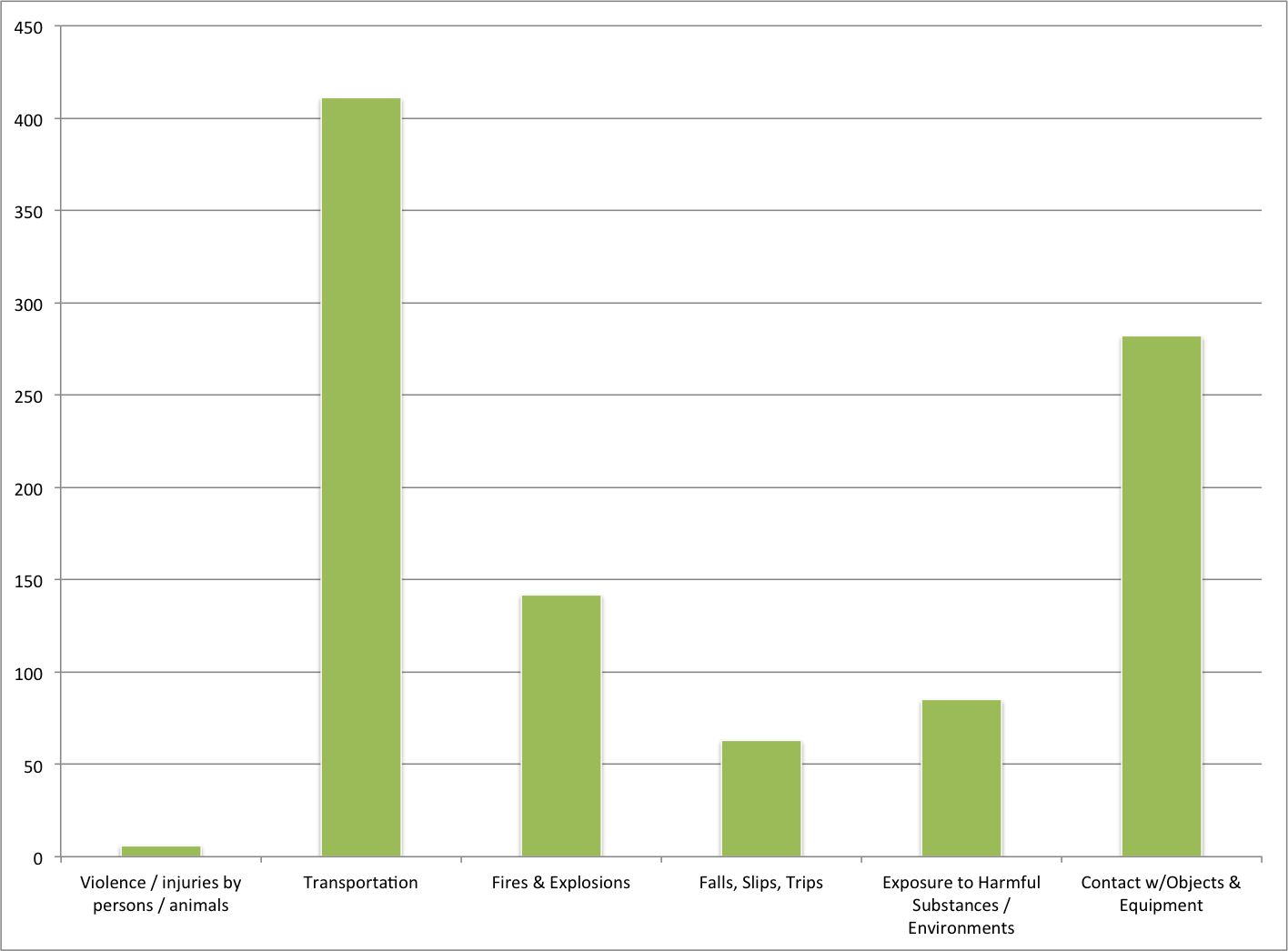
Fig. 2. Reasons for O&G Fatalities 2003-12. Aggregated from Table 1.
Like many industrial operations, here are some of the reasons why oil and gas workers may be hurt or killed according to OSHA:
Vehicle Accidents
Struck-By/ Caught-In/ Caught-Between Equipment
Explosions and Fires
Falls
Confined Spaces
Chemical Exposures
If you drill down to the raw fatality-cause numbers, you can see that the fatal worksite hazards vary over time and job type1 (Table 1, bottom). Supporting jobs to the O&G sector are at higher risk of fatal injuries than those within the O&G extraction job category2. The chart to the right shows aggregate data for years 2003-12. Records indicate that the primary risk of death originated from transportation incidents, followed by situations where someone came into contact with physical equipment (Fig. 2).
A recent NIOSH study by Esswein et al. regarding workplace safety for oil and gas workers was that the methods being employed to protect workers against respirable crystalline silica3 were not adequate. This form of silica can be found in the sand used for hydraulic fracturing operations and presents health concerns such as silicosis if inhaled over time. According to Esswein’s research, workers were being exposed to levels above the permissible exposure limit (PEL) of ~0.1 mg/m3 for pure quartz silica because of insufficient respirator use and inadequate technology controls on site. It is unclear at this time how far the dust may migrate from the well pad or sand mining site, a concern for nearby residents of the sand mines, distribution methods, and well pads. (Check out our photos of a recent frac sand mine tour.) The oil and gas industry is not the only employer that must protect people from this airborne workplace hazard. Several other classes of jobs result in exposure to silica dust above the PEL (Fig. 3).
References and Additional Resources
1. What do the job categories in the table below mean?
For the Bureau of Labor Statistics, it is important for jobs to be classified into groups to allow for better reporting/tracking. The jobs and associated numbers are assigned according to the North American Industry Classification System (NAICS).
(NAICS 21111) Oil and Gas Extraction comprises establishments primarily engaged in operating and/or developing oil and gas field properties and establishments primarily engaged in recovering liquid hydrocarbons from oil and gas field gases. Such activities may include exploration for crude petroleum and natural gas; drilling, completing, and equipping wells; operation of separators, emulsion breakers, desilting equipment, and field gathering lines for crude petroleum and natural gas; and all other activities in the preparation of oil and gas up to the point of shipment from the producing property. This industry includes the production of crude petroleum, the mining and extraction of oil from oil shale and oil sands, the production of natural gas, sulfur recovery from natural gas, and the recovery of hydrocarbon liquids from oil and gas field gases. Establishments in this industry operate oil and gas wells on their own account or for others on a contract or fee basis. Learn more
(NAICS 213111) Drilling Oil and Gas Wells comprises establishments primarily engaged in drilling oil and gas wells for others on a contract or fee basis. This industry includes contractors that specialize in spudding in, drilling in, redrilling, and directional drilling. Learn more
(NAICS 213112) Support Activities for Oil and Gas Operations comprises establishments primarily engaged in performing support activities on a contract or fee basis for oil and gas operations (except site preparation and related construction activities). Services included are exploration (except geophysical surveying and mapping); excavating slush pits and cellars, well surveying; running, cutting, and pulling casings, tubes, and rods; cementing wells, shooting wells; perforating well casings; acidizing and chemically treating wells; and cleaning out, bailing, and swabbing wells. Learn more
2. Fifteen percent of all fatal work injuries in 2012 involved contractors. Source
3. What is respirable crystalline silica?
Respirable crystalline silica – very small particles at least 100 times smaller than ordinary sand you might encounter on beaches and playgrounds – is created during work operations involving stone, rock, concrete, brick, block, mortar, and industrial sand. Exposures to respirable crystalline silica can occur when cutting, sawing, grinding, drilling, and crushing these materials. These exposures are common in brick, concrete, and pottery manufacturing operations, as well as during operations using industrial sand products, such as in foundries, sand blasting, and hydraulic fracturing (fracking) operations in the oil and gas industry.
4. OSHA Fact Sheet: OSHA’s Proposed Crystalline Silica Rule: General Industry and Maritime. Learn more
Employee health and safety are protected under the following OSHA regulations. These standards require employers to make sure that the workplace is in due order:
Oil and gas extraction industries include oil and gas extraction (NAICS 21111), drilling oil and gas wells (NAICS 213111), and support activities for oil and gas operations (NAICS 213112).
b
Data in event or exposure categories do not always add up to total fatalities due to data gaps.
c
Based on the BLS Occupational Injury and Illness Classification System (OIICS) 2.01 implemented for 2011 data forward
d
Includes violence by persons, self-inflicted injury, and attacks by animals
e
Includes highway, non-highway, air, water, rail fatal occupational injuries, and fatal occupational injuries resulting from being struck by a vehicle.
https://www.fractracker.org/a5ej20sjfwe/wp-content/uploads/2014/05/Fatality-Reasons.png10461416FracTracker Alliancehttps://www.fractracker.org/a5ej20sjfwe/wp-content/uploads/2025/09/2025-Wordmark-Logo.pngFracTracker Alliance2014-05-14 12:46:092020-07-21 10:42:26Well Worker Safety and Statistics
By Ted Auch, OH Program Coordinator, FracTracker Alliance
Ohio is the only shale gas state in the Marcellus and/or Utica Shale Basin that has decided to go “all in.” i.e. The state is moving forward with shale gas production, Class II Injection Well disposal of brine waste from fracking, and more recently the processing and disposal of drill cuttings/muds via the state’s Solid Waste Disposal (SWD) districts and waste landfills. The latter would fall under the joint ODNR, ODH, and EPA’s September 18, 2012 Solidification and Disposal Activities Associated with Drilling-Related Wastes advisory. It occurred to us that it might be time to try to estimate how much of these materials are produced here in Ohio on a per-well basis using basic math, data gleaned from Ohio’s current inventory of Utica wells and the current inventory of PLAT maps, and some broad assumptions as to the density of Ohio’s geology.
Developing the Estimate
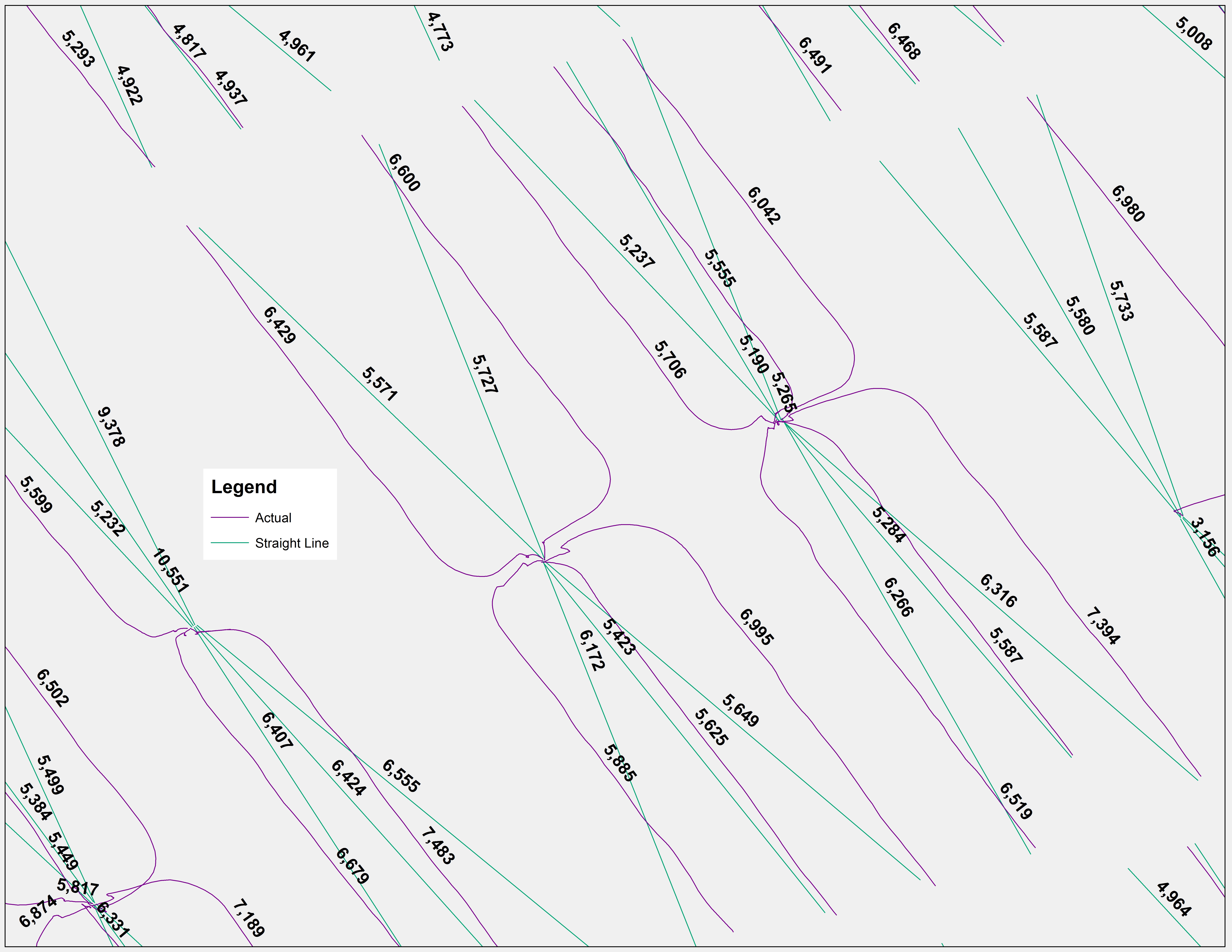
1) Start with a 341 Actual Utica well lateral dataset generated utilizing the ODNR Ohio Oil & Gas Well Database PLAT inventory or the current inventory of 1,137 permitted Utica wells. Generate a Straight Line lateral dataset by converting this data from “XY To Line” with the following summary statistics:
Average Lateral + Vertical Footage = 13,205-13,261 total feet (402,488-404,195 centimeters) (Figure 1)
Fig. 1. An example of Actual and Straight Line Utica well laterals in Southeast Carroll County, Ohio
3) We assume a rough diameter of 8″ down to 5″ (20-13 centimeters) for all of 1) and 14″ to 8″ (36-20 centimeters) for the entirety of 2)
4) The density of 1) is roughly 2.61 g cm3 assuming the average of seven regional shale formations (Manger, 1963)
5) None of the materials being drilled through are igneous or metamorphic (limestone, siltstone, sandstone, and coal) thus the density of 2) is all going to be
≈2.75 g cm3
6) The volume of the above is calculated assuming the volume of a cylinder
(i.e., V = hπr2):
Σ of Actual Lateral Length 49,205,721 cm3 * 2.61 g = 128,180,904 g
Σ of Actual Lateral Length 153,991,464 cm3 * 2.75 g = 423,476,526 g
Average Lateral + Vertical Volume = 551,657,430 grams = 1,216,195 pounds =
608 tons of drill cuttings per Utica well * 829 drilled, drilling, or producing wells = 504,113 million tons
The coarse assumptions as to density of materials and the fact that these materials experience significant increases in surface area once they have been drilled through.
The assumptions as to pipe diameter could be over or underestimating drill cuttings due to the fact that we know laterals taper as they near their endpoint. We assume 45% of the vertical depth is comprised of 14″ diameter pipe, 40% 11″ diameter pipe, and 15% 8″ pipe. Similarly we assume the same percentage distribution for 8″, 6.5″, and 5″ lateral pipe.
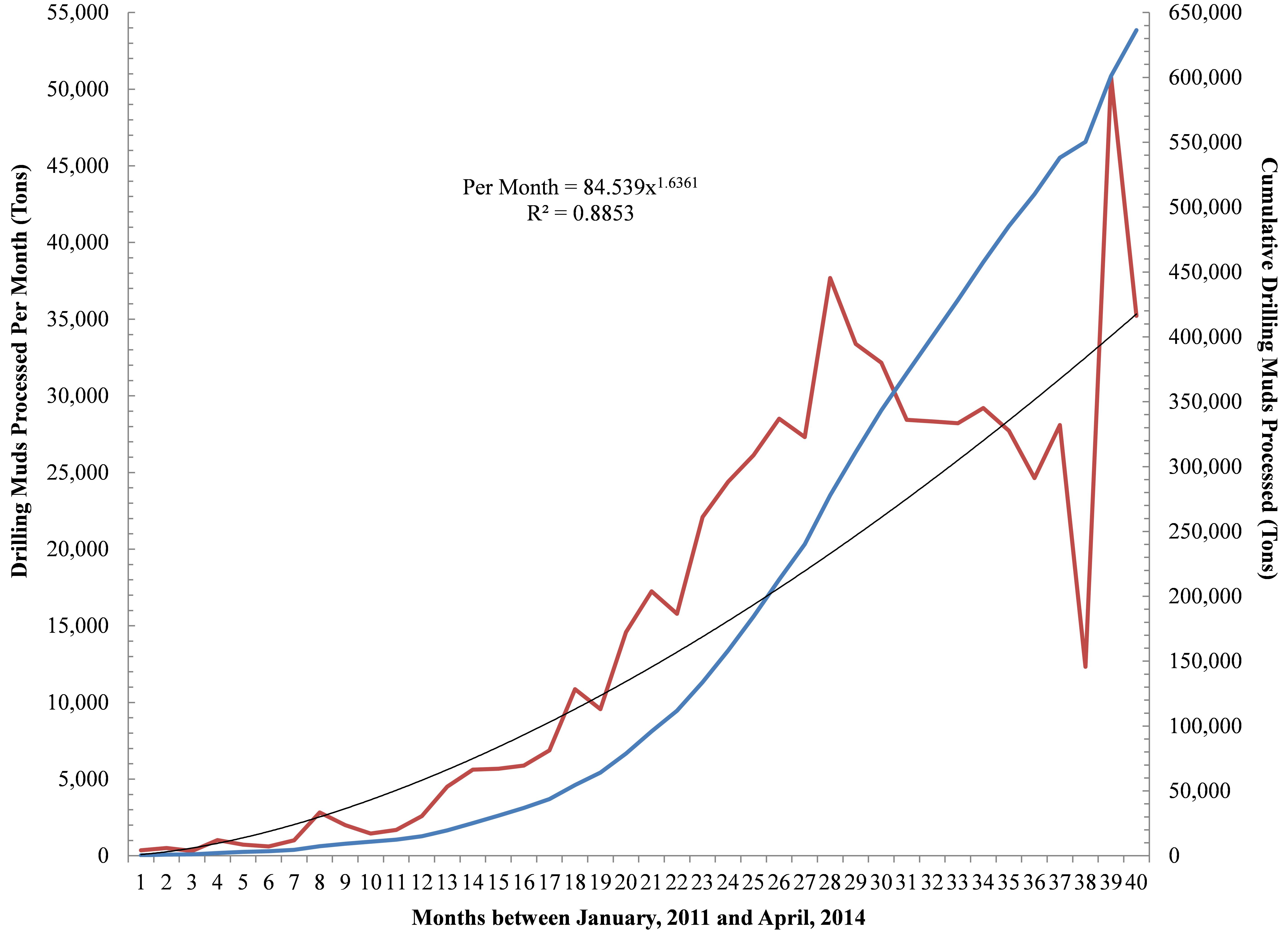
Ohio Drilling Mud Generation and Processing
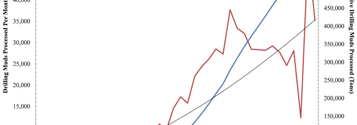
Fig. 2. Month-to-month and cumulative drilling muds processed by CCHSWD, one of six OH SWDs charged with processing shale gas drilling waste from OH, WV, and PA.
Ohio’s primary SWDs responsible for handling the above waste streams – from in state as well as from Pennsylvania and West Virginia – are the six southeastern SWDs along with the counties of Portage and Mahoning according to several anonymous sources. However, when attempting to acquire numbers that speak to the flows/stocks of fracking related SWD waste (i.e., drilling muds) the only district that keeps track of this data is the Carroll-Columbiana-Harrison Solid Waste District (CCHSWD). The CCHSWD’s Director of Administration was generous enough to provide us with this data. According to a month-over-month analysis they have processed 636,450 tons generating a fixed fee of $3.5 per ton or $2.23 million to date (Figure 2). This trend translates into a 1,046-1,571 ton monthly increase depending on how you fit your trend line to the data (i.e., linear Vs power functions) or put another way annual drilling mud increases of 12,546-18,847 tons.
https://www.fractracker.org/a5ej20sjfwe/wp-content/uploads/2014/05/SWD_DrillingMuds-scaled.jpg10891500Ted Auch, PhDhttps://www.fractracker.org/a5ej20sjfwe/wp-content/uploads/2025/09/2025-Wordmark-Logo.pngTed Auch, PhD2014-05-08 13:36:222020-07-21 10:42:26Utica Shale Drill Cuttings Production – Back of the Envelope Recipe
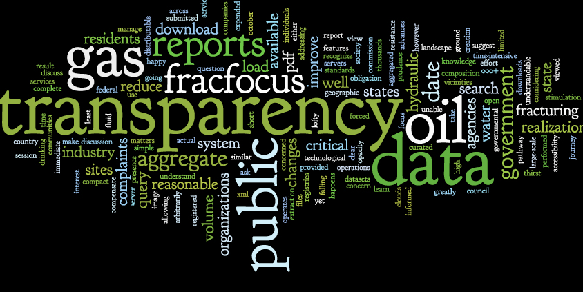
FracFocus.org is the preferred chemical disclosure registry for the oil and gas (O&G) industry, and use of your website by the industry is mandated by some states and regulatory agencies. As such, we hope you’ll be responsive to this call by FracTracker, other organizations, and concerned citizens across the country to live up to the standards of accessibility and transparency required by similar data registries.
A Focus on Data Transparency
Recent technological advances in high volume hydraulic fracturing operations have changed the landscape of O&G drilling in the United States. As residents adjust to the presence of large-scale industrial sites appearing in their communities, the public’s thirst for knowledge about what is going on is both understandable and reasonable. The creation of FracFocus was a critical first step down the pathway to government and industry transparency, allowing for some residents to learn about the chemicals being used in their immediate vicinities. The journey, however, is not yet complete.
Design Limitations on FracFocus
Query by Date
Even with the recently added search features there is no way to query reports by date. Currently a visitor would be unable to search by the date hydraulic fracturing / stimulation was performed, or when the report itself was submitted. Reports can only be viewed one PDF at a time, which would take someone quite a while to view all 68,000+ well sites in your system.
Aggregate Data Downloads
In October 2013, you informed us that “each registered state regulatory agency has access to the xml files for their state but they are not distributable from FracFocus to the public.” We must ask the reasonable question of “why not?” We understand that setting up a downloadable data system is a time-intensive process, as we manage one ourselves, but the benefits of providing such a service more than compensate for the effort expended. It is no longer possible to aggregate data, either automatically or manually, because of bandwidth limitations that keep users from downloading more than an arbitrarily limited number of reports in a single session. Considering public concern over the composition of frac fluid, as well as the volume and geographic extent of complaints of drinking water complaints to be related to O&G extraction, prudence would suggest making the data as accessible as possible. For example, making the aggregated data available to the public as a machine-readable download would greatly reduce the load on your servers, because users would no longer be forced to download the individual PDF reports. Changes in the way the reports are curated would also improve efficiency and reduce your server load; we would be more than happy to discuss these changes with you.
An Issue of Money?
The basic infrastructure to provide this service via FracFocus.org is already in place. An organization like the Groundwater Protection Council with a website serving some of the world’s wealthiest corporations loses credibility when making claims that “we have no way to meet your needs for the data.” Withholding data from the public only serves to compound the distrust that many people have with regards to the oil and gas extraction industry. Additionally, agencies that use FracFocus as a means of satisfying open government requirements are currently being short changed by the lack of access to your aggregated datasets; restricting access to data that is in the public interest is fundamentally at odds with data transparency initiatives, including the President’s 2013 Executive Order on Open Data.
One Small Step for a Company…
Within this discussion is a simple realization: The Ground Water Protection Council, Interstate Oil and Gas Compact Commission, participating companies and states, and the federal government should recognize that data transparency is not merely a lofty ideal, but an actual obligation to our open society. Once that realization has been made, the path of least resistance becomes clear: you, FracFocus, should make all of your aggregate data available to the public, beginning with the easiest step: the statewide datasets that are already being provided to government agencies.
FracTracker operates in the public interest. We – and the thousands of individuals and organizations who use our services and yours – request no less from you. Thank you for addressing these critical matters.
Sincerely, -The FracTracker Alliance-
https://www.fractracker.org/a5ej20sjfwe/wp-content/uploads/2014/04/FF-Word-Cloud.png522844FracTracker Alliancehttps://www.fractracker.org/a5ej20sjfwe/wp-content/uploads/2025/09/2025-Wordmark-Logo.pngFracTracker Alliance2014-04-30 09:00:082020-07-21 10:42:25An Open Letter to FracFocus
By Ted Auch, OH Program Coordinator, FracTracker Alliance
The “Why?”
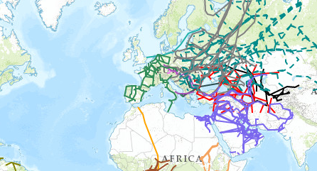
Recently, the US has proposed to ship American shale gas abroad to buffer Europe’s 15-30% reliance on Russian gas imports in the face of the annexation of Crimea by Russia – and parallel 80% increases in LNG prices paid by Eastern Europeans to Russia’s Gazprom. The FracTracker map below illustrates all proposed and existing hydrocarbon pipelines across South America, Africa, Europe, the Persian Gulf, and Asia/Russia1. Creating such a map seems the least we could do given that this conflict has been called the “worst crisis with the West since the end of the Cold War.” The situation in Crimea is a chronic crisis; folks like Oxford University’s Jonathan Stern have suggested:
Ukraine owes Gazprom $2 billion for already delivered hydrocarbons,
Russia can easily turn their supplies to Japan which will pay a premium relative to what they are getting from the European Union, and
The duration of European oil and gas contracts with Gazprom, which extend 15-35 years, can’t be broken (Einhorn, 2014; Henderson and Stern, 2014).
The rhetoric framing here in the US has been lead by – and regurgitated by media outlets such as NPR who suggested “Putin Could Send Europe Scrambling For Energy Sources” – the likes of the Council on Foreign Relations Richard Haass and the Brookings Institution’s Bruce Jones. Both of these entities have the ears of congress domestically and global decision makers at gatherings such as the World Economic Forum in Davos, Switzerland (Gwertzman, 2014; Wade and Rascoe, 2014).
Stepping up hydrocarbon and extraction technologies is not universally espoused:
This is not an immediate-term solution. It’s not even an intermediate-term solution. – Paul Bledsoe, German Marshal Fund, in The New York Times
Originally, shale gas production was proposed as a way for the US to become “energy independent,” but the dogma has rapidly and in a coordinated fashion shifted to the export of shale gas itself and the technology used to get it out of the ground. This rhetoric is now the focus not just of Washington, DC think tanks but academics (Bordoff, 2014) .
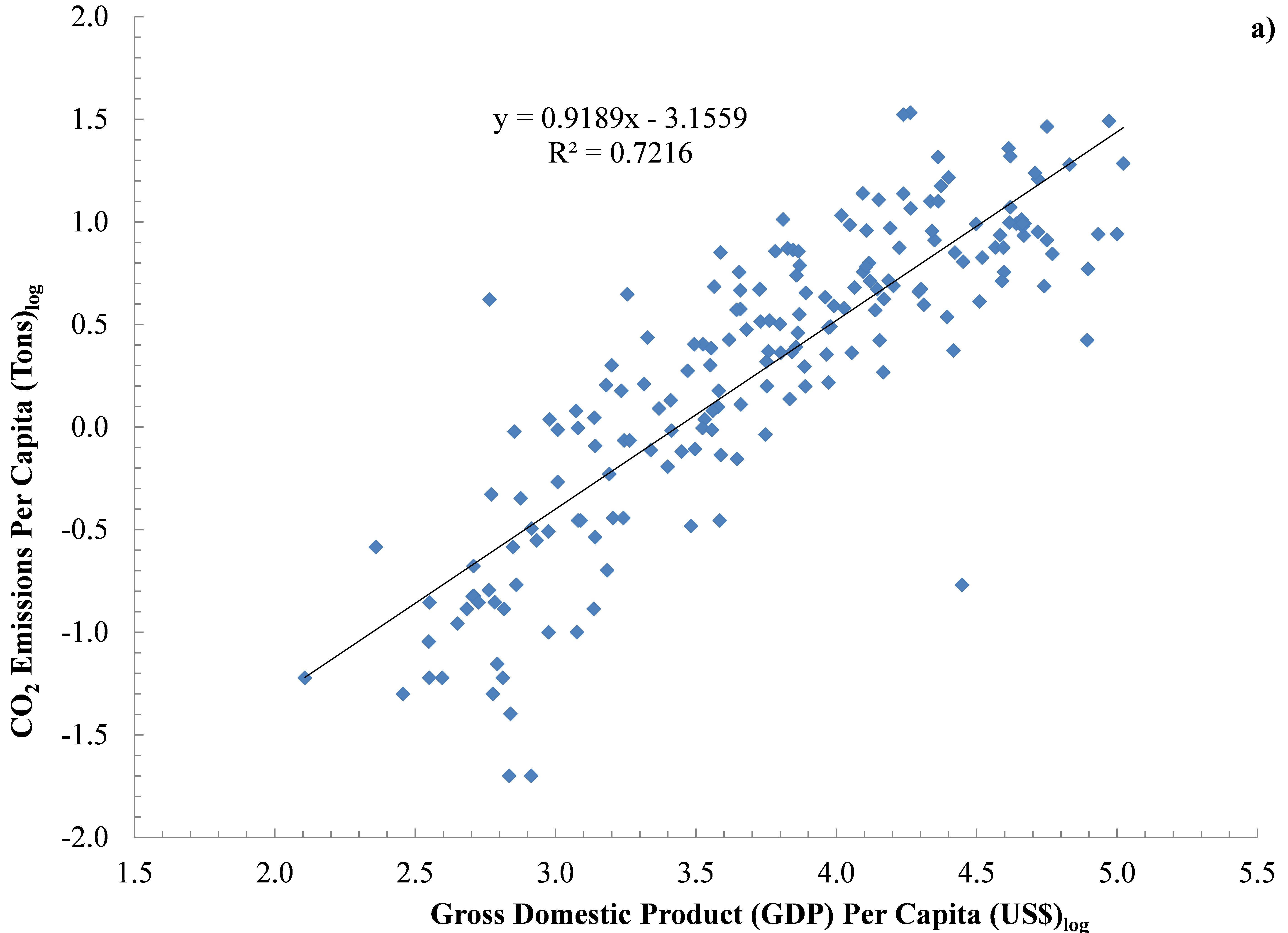
Figure 1a) Global CO2 Per Capita Emissions (Tons) Vs Per Capita Gross Domestic Product (GDP) (US $)
The above regions are ripe for – or currently experiencing – significant political uprisings from the Niger Delta and Venezuela to the percolating anger associated with increasing economic stratification and political elite disconnect in countries like Saudi Arabia, Libya, Yemen, Pakistan, Mediterranean Africa writ large, Sudan, and Oman2. Often this discontent is emanating out of citizens’ concerns as to where oil revenues are going and how often the hydrocarbon largesse is concentrated in a handful of political elites and/or oligarchs (Nossiter, 2014). The EIA estimates Russia and China sit atop an estimated 107 billion barrels of shale oil and 1,400 TCF of shale gas. Much of this resource will be required if they are to continue > 2-5% Gross Domestic Product (GDP) growth. The remainder they will undoubtedly use as a cudgel to deflect the west’s suggestions and/or demands within their borders or their “near abroad.” In the case of Russia, the “near abroad” generally refers to the eight former Communist pliable nations – and are incidentally home to nontrivial shale oil and gas reserves – that act as a physical and ideological buffer between them and NATO/European Union states. In an effort to combat the asymmetric hydrocarbon supply and demand issues and secure access to the sizable shale reserves in eastern Europe, the European Union continues to push the European Neighborhood Policy meant to create a “ring of friends”3 – with Ukraine just the latest significant test and the only successes being Tunisia and Moldova (Charlemagne, 2014). With respect to China, their “near abroad” nations include shale oil and gas rich nations like Indonesia, Thailand, Myanmar, Cambodia, and Vietnam, along with ex-Soviet region Central Asian countries which provide China with 80% of its natural gas needs. However, the east-west tug of war has come down to the willingness of the east to offer larger instant loans, cheaper gas, and labor/technology needed to develop pipeline networks. The nexus between these two eastern giants is the proposed – and recently agreed upon – $400 billion Sino-Russian energy cooperation natural gas and oil pipeline. This proposal will stretch across heretofore relatively undisturbed and isolated communities and the ecosystems they have evolved with across the Eurasian Steppe and Siberia (Einhorn, 2014).
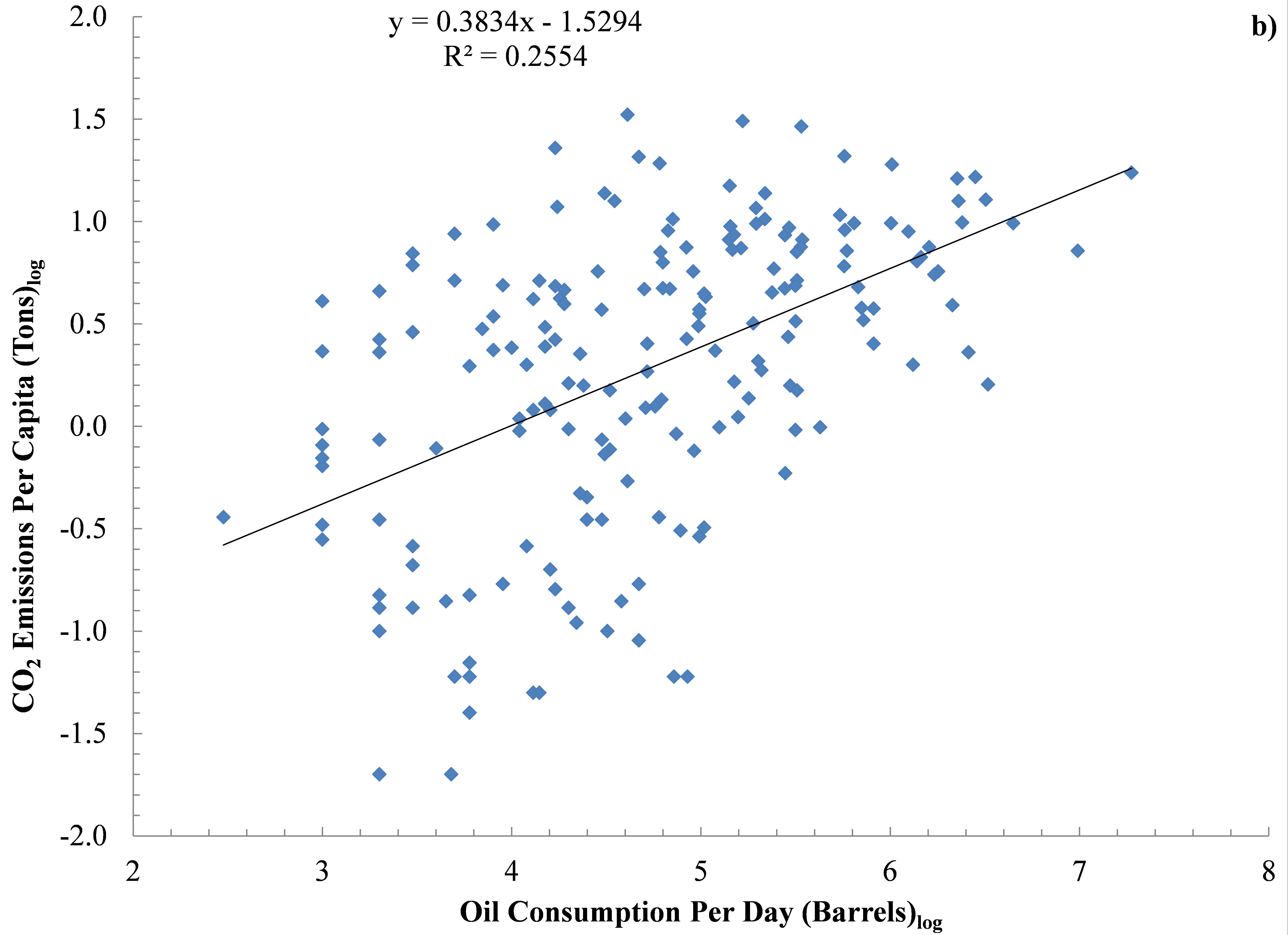
Figure 1b) Global CO2 Per Capita Emissions (Tons) Vs Oil Consumption Per Day (Barrels) across 204 countries
The fomenting anger and geopolitical combativeness that result from these conditions put the global hydrocarbon transport network at risk. Analogies to R.A. Radford’s The Economic Organization of a P.O.W. Camp can be made here, where the economy that Mr. Radford created flourished until the input stream from the Red Cross stopped. It was at this time that the economy collapsed due to its singular reliance on one input source. Similar analogies exist across emerging, P5+1, and frontier markets worldwide, with many countries largely dependent upon hydrocarbon imports or exports to stoke GDP. Such imports, along with oil consumption, account for 98% of per country CO2 emissions (Table 1 below, Figure 1a-b). Revolution or even temporary and targeted political instability will fuel the type of hydrocarbon transport/production disruption that will produce the kind of jump condition described by Mr. Radford. A jump condition occurs in situations when suitable hydrocarbon stocks/flows are lost, pipelines are turned off, and alternative transport channels are deemed too perilous. Such a crisis is one that no industrialized or industrializing nation is prepared to manage, making the 2007-08 Financial Crisis look and feel like child’s play. Thus, many private and state actors are proposing new and expanded hydrocarbon pipeline networks to reduce reliance on single-large networks emanating from or traveling through volatile regions. Proposals range from the large Nabucco pipeline proposal connecting Asia and Europe or the Nord Stream AG Baltic Sea Gas Pipeline to small regional or inter-state proposals in Africa, the Persian Gulf, and Eastern Europe.
The “When?”
With this map, which was initiated in January 2014, we have attempted to accurately quantify as many existing and proposed pipeline routes as possible in Europe, Africa, South America, Asia, and the Persian Gulf. We will be updating this map periodically, and it should be noted that all layers are predetermined aggregations of regional pipelines. Given the recent EIA global shale oil and gas estimates, it is only a matter of time before: a) European nations like Germany, Ukraine, Poland, and Romania begin to explore shale gas extraction in the name of “energy independence,” and b) Argentina hands over the proverbial keys to its 16.2-22.5 billion barrels of oil in the Vaca Muerta shale basin to the likes of Shell or Repsol-YPF (Canty, 2011; Gonzalez and Cancel, 2013; Romero and Krauss, 2013; Staff, 2013). This conversation will be accompanied by additional pipeline proposals for inter- and intra-region transport, all of which we will incorporate into this map on a quarterly basis. If you know of proposals that are not currently shown on the map, please let us know.
Table 1. Major Worldwide Flows of Oil (Thousand Barrels Per Day).
Bordoff, J., 2014. Adding Fuel to the Fire: How the American shale gas boom can weaken Russia’s hand in Ukraine, Foreign Policy Magazine, Washington, DC.
Canty, D., 2011. Repsol hails largest ever 927 million bbl oil find, ArabianOilandGas.com. ITP Business Portal.
Charlemagne, 2014. How to be good neighbours: Ukraine is the biggest test of the EU’s policy towards countries on its borderlands, The Economist, London, UK.
Einhorn, B., 2014. How the Ukraine Crisis Could Help Clear Beijing’s Smog, Bloomberg Businessweek. Bloomberg LP, New York, NY.
Gonzalez, P., Cancel, D., 2013. Shell to Triple Argentine Shale Spending as Winds Change, Bloomberg Magazine. Bloomberg LP, New York, NY.
Gwertzman, B., 2014. How to respond to Ukraine’s Crisis, Council on Foreign Relations, Washington, DC.
Henderson, J., Stern, J., 2014. The Potential Impact on Asia Gas Markets of Russia’s Eastern Gas Strategy, Oxford Energy Comment. The Oxford Institute for Energy Studies, Oxford, UK, p. 13.
Klein, N., 2008. The Shock Doctrine: The Rise of Disaster Capitalism. Picador.
Klein, N., 2014. Why US Fracking Companies Are Licking Their Lips Over Ukraine: From climate change to Crimea, the natural gas industry is supreme at exploiting crisis for private gain – what I call the shock doctrine, The Guardian, London, UK.
Krauss, C., 2014. U.S. Gas Tantalizes Europe, but It’s Not a Quick Fix, The New York Times, New York, NY.
McDonnell, A., 2014. Fracking is unlikely to reduce gas prices to the extent its proponents desire, The London School of Economics and Political Science – British Politics and Policy. The London School of Economics, London, UK.
Nossiter, A., 2014. Nigerians Ask Why Oil Funds Are Missing, The New York Times, New York, NY.
Romero, S., Krauss, C., 2013. An Odd Alliance in Patagonia, The New York Times, New York, NY.
Staff, 2013. Argentina’s YPF: Swallowed Pride, The Economist, London, UK.
Wade, T., Rascoe, A., 2014. Global gas trade may soften foreign policy of Russia, China, Reuters, New York, NY.
[2] The EIA estimates Mediterranean Africa contains 5,772 TCF of estimated wet shale natural gas and 1,373,770 million barrels of oil, the Former Soviet Union 4,738 TCF and 310,567 million barrels, and South America 2,465 TCF and 643,864 million barrels 73% of which is in Brazil and Argentina’s Vaca Muerta.
[3] According to The Economist “The Europeans should also rethink the neighbourhood policy, which lumps together disparate countries merely because they happen to be nearby. In the south it may have to devise a wider concept of its interests stretching out to the Sahel, the Horn of Africa and the Middle East. Here Europe has no real friends, lots of acquaintances and not a few enemies. To the east it needs better ways of helping those who want to move closer to the EU.”