The Muskingum Watershed and Utica Shale Water Demands
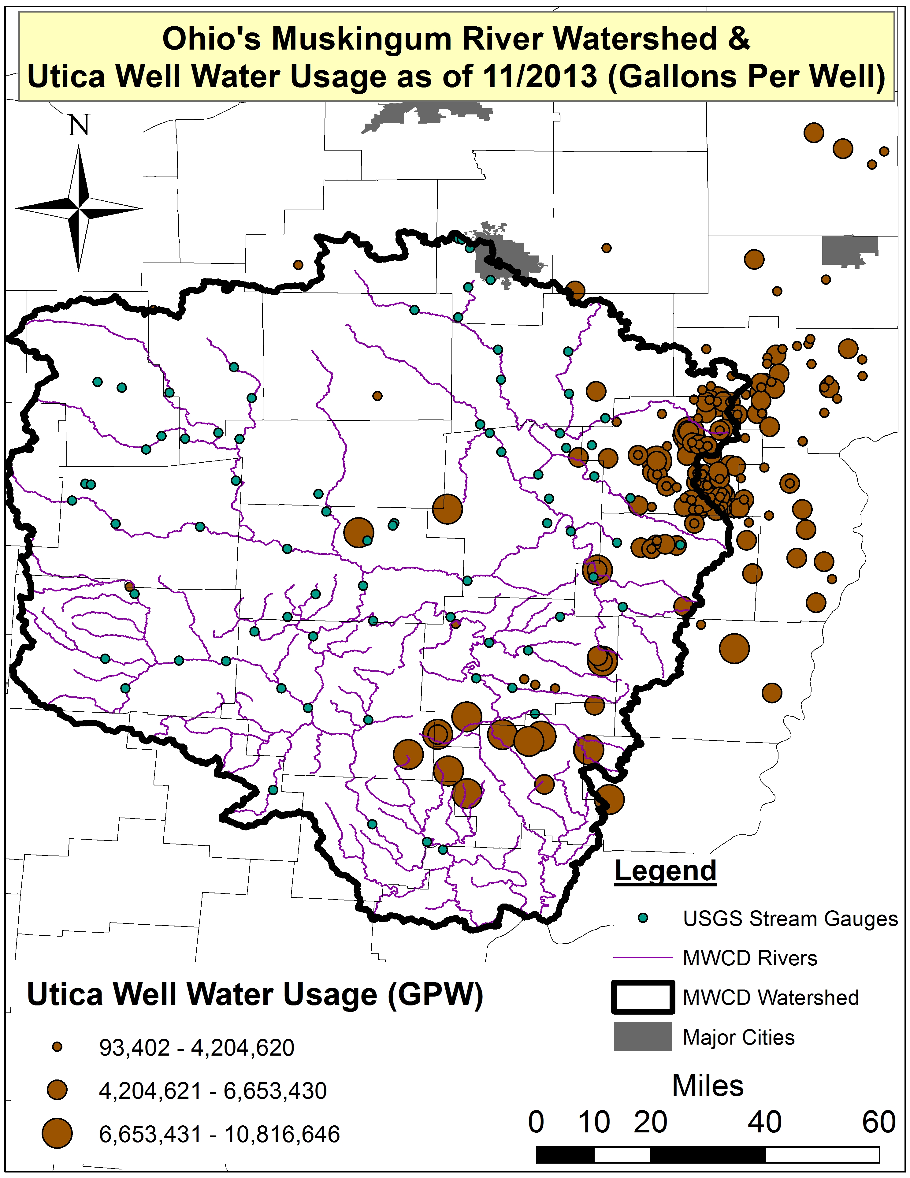
Figure 1. Ohio Utica well water usage across 306 wells (Gallons Per Well)
How much freshwater has the unconventional drilling industry used to-date?
By Ted Auch, OH Program Coordinator, FracTracker Alliance
Given that Ohio’s largest conservancy district, the Muskingum Watershed Conservancy (MWCD), is considering the sale of large stocks of freshwater and deep mineral rights to the Utica Shale drilling industry, we thought it would be helpful to take a “back of the envelope” first look at how much freshwater the gas industry has already used within the basin and how much it might use given current permitting trends.
Background
But first a little background… The MWCD is an 18 county political body that encompasses the Muskingum River basin in its entirety – roughly 19% of the state’s landmass (Figure 1). The Muskingum River Watershed (MRW), Ohio’s “largest wholly contained watershed,” contains nearly 19% of OH’s wetlands and 28% of the state’s lakes and reservoirs (Table 1).
| Table 1. The number, minimum/maximum size, total area, and mean (±) size of wetlands, lakes, and reservoirs in the Muskingum River Watershed (MRW) | ||||||
|
# |
Min |
Max |
Sum |
Mean |
± |
|
|
Wetlands (acres) |
||||||
|
MRW |
25,529 |
0.014 |
507 |
98,924 |
3.87 |
12.01 |
|
Ohio River |
134,736 |
6.9*10-5 |
1,500 |
507,312 |
3.77 |
13.94 |
|
MRW as % of Ohio |
18.9 |
202.9 |
33.8 |
19.5 |
102.7 |
86.2 |
|
Lakes & Reservoirs (miles2) |
||||||
|
MRW |
25 |
0.35 |
5.5 |
44.6 |
1.78 |
1.5 |
|
Ohio River |
91 |
0.15 |
5,014 |
5,545 |
61 |
523 |
|
MRW as % of Ohio |
27.5 |
233.3 |
0.1 |
0.8 |
2.9 |
0.3 |
The sustainability of the watershed’s freshwater stocks and flows is of concern to many, given climate trends and the fact that the MWCD, according to their website, is “…awaiting results from a U.S. Geological Survey analysis of water availability at several other reservoirs before deciding whether to approve a growing number of requests for water by other drilling companies.”
Water Use Trend
Our methodology examined rainfall, evapotranspiration, and usage of water by forests, crops, and humans. “When we account for all of these usages, as well as unquantified usages like watershed discharge and soil holding capacity, the remainder is what I will call available water.”
According to our analysis of 306 drilling, drilled, or producing OH Utica gas wells, the hydraulic fracturing process requires on average 4.6-4.8 million gallons of water per well(2). This is equal to 2.8-2.9 billion gallons of water to-date for the watershed’s 613 wells or 4.5-4.7 billion gallons across the state’s currently permitted 985 wells (Figure 1).
After looking at water use from this industry, the following water usage scenarios emerge:
- For just Muskingum Watershed gas wells – water use is equivalent to 2.47% of the watershed’s “available water” assuming a low discharge scenario, 2.50% for a medium discharge scenario, and 2.56% for a high discharge scenario.
- For all Utica gas wells in Ohio – water use is equivalent to 3.97% of the watershed’s “available water” assuming a low discharge scenario, 4.02% for a medium discharge scenario, and 4.11% for a high discharge scenario.
| Put another way, these volumes equate to 4.44 and 7.14% of Muskingum Watershed residences’ total annual water usage. |
A year from now – assuming two Utica permitting trajectories(3) – our calculations resulted in the following estimates:
(Note: The below projections assume the entirety of Ohio Utica wells permitted to date or 985 permits and an increase in Utica Well water usage of 220,329 gallons per quarter(4).)
- 25 permits per month for the next 12 months – equivalent to 5.40, 5.47, or 5.59% of the watershed’s “available water” by November 2014 when added to the currently utilized water detailed in part 1 above. This will be equivalent to 9.70% of human water usage in Ohio.
- 51 permits per month for the next 12 months – equivalent to 6.90, 7.00, or 7.14% of the watershed’s “available water”. This will equal 12.40% of human annual water usage in the watershed.
Ohio vs. Other States
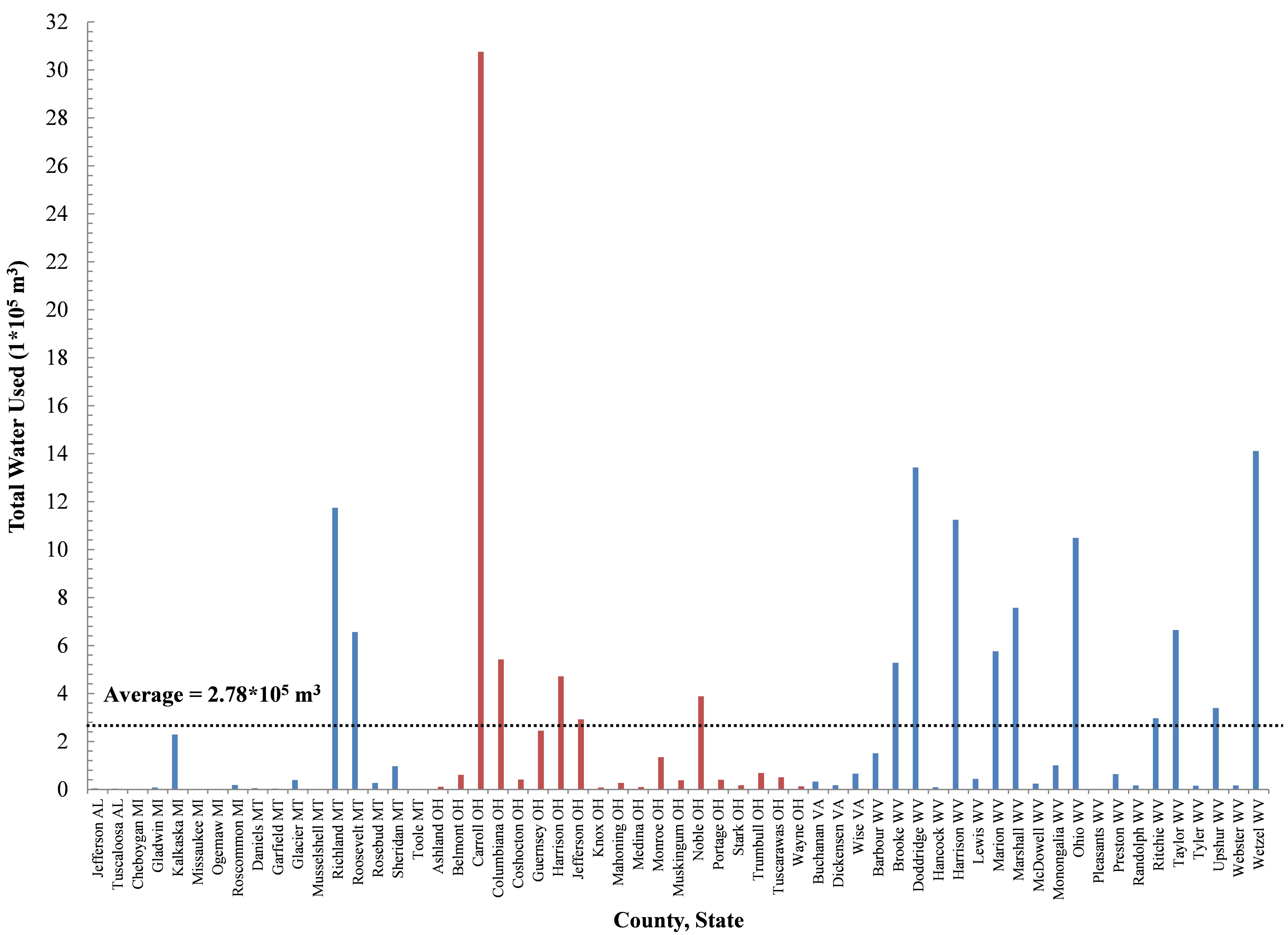
Figure 2. Total horizontal drilling water usage across 59 Counties in 6 US states (1*105 m3)
To put OH into perspective, we decided to compare the above water usage across 19 OH counties to identical data for 40 counties in 5 other states. In doing so we found that each county’s horizontal well stock has used an average of 2.82*105 m3 of water to date or 3,912 swimming pools and 119 golf course acres worth of irrigation, with the latter equivalent to 1.53 US golf courses. Six of OH’s counties come in over this average and the remaining thirteen below. Meanwhile, 10 of neighboring West Virginia’s 19 counties exceeded 2.79*105 m3 of water. OH and WV horizontal well water usage averaged across counties exceeds the Six State*Fifty-Nine County continuum average by 0.13 and 1.48*105 m3 of water, while the remaining four states fall short of the average by 2.02*105 m3 (Figure 2).
Total water usage across the 59 counties turns out to be a robust predictor of how the industry’s water needs relate to general public water usage accounting for 78.4% of the latter (Figure 3). However, this relationship isn’t as straightforward as one might expect – requiring a statistical technique called log transformation which is generally applied by statisticians to data that is “highly skewed…This can be valuable both for making patterns in the data more interpretable and for helping to meet the assumptions of inferential statistics.” Due to the “skewness” of this data set, the average and median industry water usage as a percent of the general public is 1.40% and 11.83%, respectively.
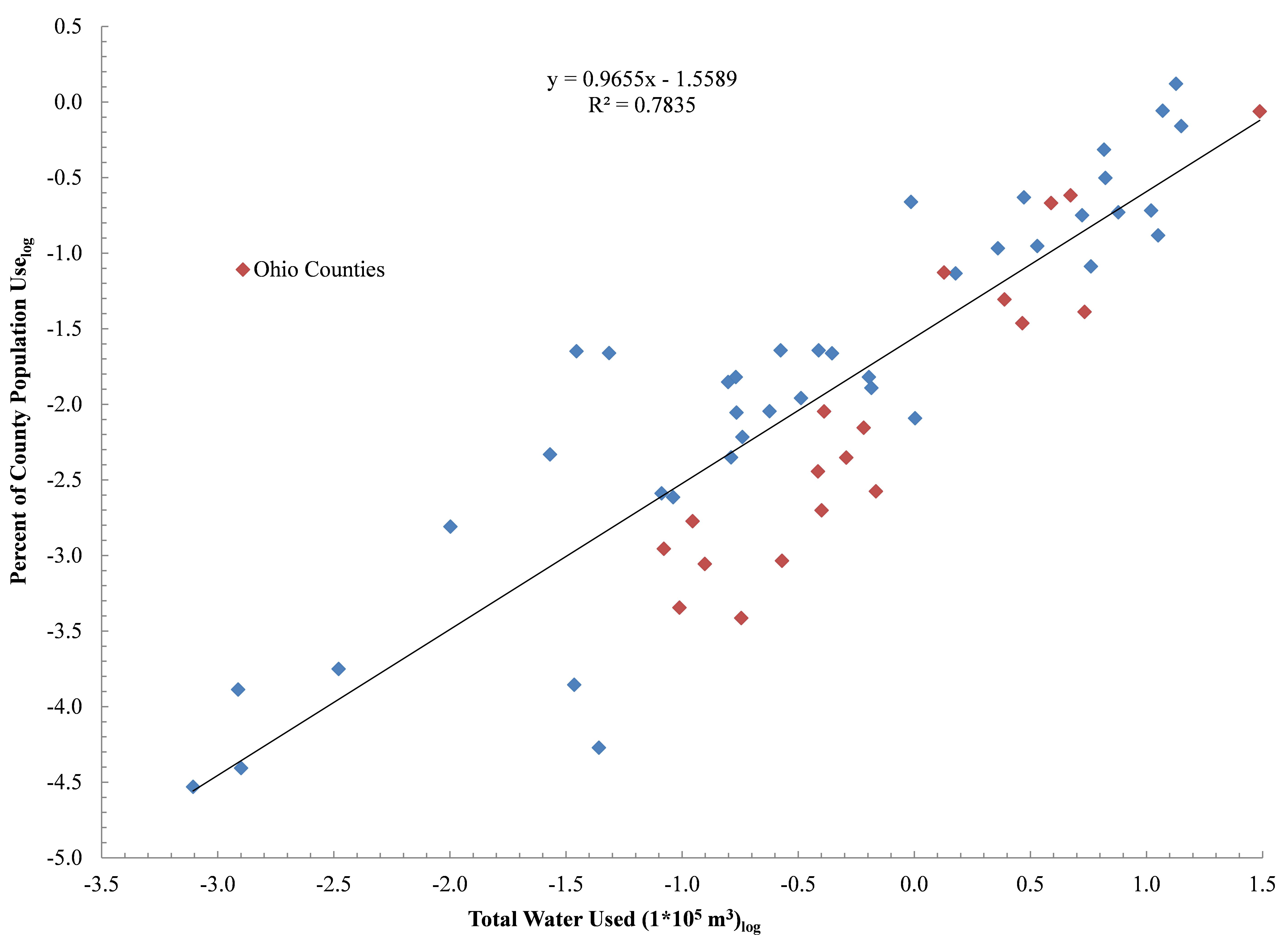
Figure 3. Total horizontal drilling water usage across 59 Counties in 6 US states relative to the general public’s water requirements (1*105 m3)
OH Inter-County Utica Water Usage By The Numbers
Hydraulic Fracturing Industry Yearly Water Usage
- Per well – 5.29 million gallons (Note: This is increasing by 149-220K gallons per quarter)
- Total water usage is increasing by 36.993 million gallons per quarter, which means that within 5-6 years the industry will be using more than 1.1 billion gallons of freshwater per year
- Per Square Mile – 10,355 gallons
- Per Capita – 138 gallons Per Well Per Person; 2,612 gallons Per Person
- Per Household – 358 gallons Per Well Per Household; 6,674 gallons Per Household
- Per Well Foot – 821 gallons
- Water Costs Per Well – $21,494 (Per capita resident water costs are $107.86 per year)
- Water Usage as a % of Total Well development and production costs – 4.41%
- The Ratio of Water as a % of Total Materials Used Per Well To Water Cost Per well – 27.25
Resident-to-Industry Ratios
- a. Per Capita Resident Water Usage Per Year as % of Per Well Usage – 0.87%
- b. Per Capita Water Cost Per Year as % of Utica Well Water Cost – 10.05%
- Ratio of (b) to (a) – 11.86
References
[1] “The Muskingum River Watershed is comprised of three major subwatersheds – the Tuscarawas River Watershed in the northeastern, the Walhonding River Watershed in the northwest and the Lower Muskingum Watershed in the south. The Tuscarawas and Walhonding rivers flow in a southern direction where they intersect at Coshocton, forming the Muskingum River.” Learn more
[2] The median per well volumes required in Oklahoma range from 3.0 million gallons for the state in totol to 4.2 million gallons for the state’s Woodford Shale horizontal wells according to a study by Kyle Murray at the University of Oklahoma.
[3] The two trajectories assume 25 and 51 permitted wells per month based on the entirety of Ohio’s Utica permitting period back to September, 2010 and the current 2013 year-to-date average, respectively.
[4] This number increases to 339,812 gallons per quarter if we remove Q3-2013 where our data is admittedly incomplete relative to the previous eight quarters. We did not include Q3-2010 or Q1 and Q2-20111 in our extrapolation because we only have data for 1, 2, and 2 wells, respectively.
[5] Mekonnen, M M, & Hoekstra, A Y. (2010). The green, blue and grey water footprint of crops and derived crop products Value of Water (Vol. 47). New York, NY: United Nations Educational, Scientific and Cultural Organization – Institute for Water Education (UNESCO-IHE).
[6] Sanford, W E, & Selnick, D L. (2013). Estimation of evapotranspiration across the conterminous United States using a regression with climate and land-cover data. Journal of the American Water Resources Association, 49(1), 217-230.
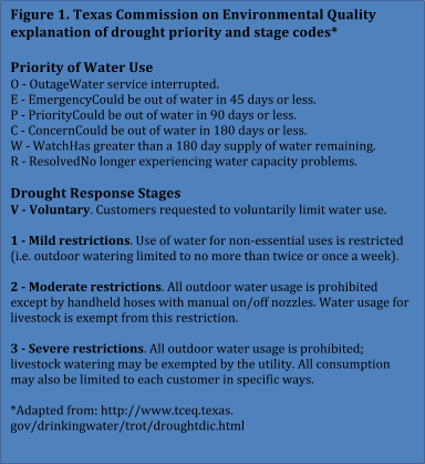 The Texas Commission on Environmental Quality, the state’s oil and gas regulatory agency, publishes