Access to reliable data is crucial to our understanding of risky fracking waste disposal, and in turn, our ability to protect public health. But when it comes to oil and gas liquid waste disposal wells in Pennsylvania, despite monitoring by two separate agencies, we are left with an incomplete and inaccurate account.
If we were to emulate the Charles Dickens classic, this article might begin, “It was the best of datasets, it was the worst of datasets.” Unfortunately, even that would be too generous when it comes to describing available data around oil and gas liquid waste disposal wells in Pennsylvania. To fully understand the legacy and current state of these wells, it is necessary to query the two agencies that have a role in overseeing them, the United States Environmental Protection Agency (EPA) and the Pennsylvania Department of Environmental Protection (DEP).
Given the relatively small inventory of these wells compared to other oil and gas producing states, the problems with the two datasets are enormous. Before jumping into these issues, however, it would be useful to review the nature of these wells, why there are two regulatory agencies involved, and why there are so few of them in Pennsylvania in the first place, relatively speaking.
Disposal Wells Categories
To further our industrial exploits of the planet, humans have found it useful to inject all kinds of things into the earth. In the United States, this ultimately falls under the jurisdiction of EPA’s Underground Injection Control (UIC) program, and the point of injection is known as an injection well. Altogether, there are six classes of injection wells, with those related to oil and gas operations falling into Class II.
There are three categories of Class II injection wells, including waste disposal, enhanced recovery, and hydrocarbon storage. There is also an infamous exemption known as the “Haliburton Loophole,” which has allowed oil and gas companies to inject millions of gallons of hydraulic fracturing fluid into oil and gas wells in order to stimulate production without any federal oversight at all.
When most people speak of “injection wells” in an oil and gas context, they are usually referring to waste disposal wells, and this is our focus here. This well type is also referred to as Class II-D (disposal) and salt water disposal wells (SWD). This latter term is used by a majority of state regulators, so we will use that abbreviation here, even though considering this type of toxic and radioactive fluid “salt water” is surely one of the industry’s most egregious euphemisms.
Dealing with Dangerous Fluids
There are two main types of liquid waste that are disposed of at SWD injection wells. As always, these waste types have a number of different names to keep everyone on their toes but for the sake of simplicity will call them “flowback” and “brine,” and both are problematic materials to handle. Additionally, the very act of industrial-scale fluid injection presents problems in its own right.
As mentioned above, when operators pump a toxic stew of water, sand, and chemicals into a well to stimulate oil and gas production, that mixture is known as hydraulic fracturing fluid, or fracking fluid. Some of these chemicals are so secretive that even the operators of the well don’t know what is included in the mix, let alone nearby residents or first responders in the event of an incident.
Between 10% and 100% of this fluid will return to the surface, and is then known as flowback fluid, becoming a waste stream. In Pennsylvania, the average amount of fracking fluid injected into production wells exceeds 10 million gallons in recent years according to data from the industry’s self-reporting registry known as FracFocus. With more than 12,000 of these wells drilled statewide, disposing of this waste stream becomes an enormous concern.
In addition to flowback fluid, there are pockets of ancient fluids encountered by the drilling and fracking processes that return to surface as well. These solutions are commonly referred to as brine due to their extremely high salt content, although this is not the type of fluid that you’d want to baste a Thanksgiving turkey with. Total salt concentrations can reach up to 343 grams per liter, roughly ten times the salt concentration of sea water. These brines include but are not limited to the familiar sodium chloride that we use to season our food, but include other components as well, including significant bromide and radium concentrations.
When Pennsylvania experimented with our public health by authorizing disposal of these fracking brines in municipal plants designed to treat sewer sludge, the bromides in that drilling waste stream became problematic as they interacted with disinfectants to cause a cancerous class of chemicals known as trihalomethanes. This ended the practice of surface “treatment” from these sites into streams in 2011, and along the way caused many water authorities to switch from chlorine to chloramine disinfectant processes. This, in turn, may have exacerbated lead exposure issues in the region, as the water disinfected with chloramine often eats away at the calcium scale deposits covering lead pipes and solder in the region’s older homes.
Marcellus and Utica wastewater are also very high in a radioactive isotope of radium known as Ra-226, which has a half-life of 1600 years. After that amount of time, half of the present radium will have emitted an alpha particle, which can cause mutations in strands of DNA when introduced inside the body, through contaminated drinking water, for example. After the hazardous expulsion of the alpha particle, the result become radon gas, which is estimated to cause 20,000 lung cancer deaths per year in the United States. Further down the decay chain is Polonium 210, which was infamously used in the assassination of Russian spy Alexander Litvinenko in London in 2006.
None of this should be injected into formations beneath people’s homes, near drinking water supplies, streams, or really anywhere that we aren’t comfortable sacrificing for the next few thousand years.
On top of all the problems with the water chemistry of both produced water and brine, the very act of injecting these fluids into the ground has triggered a large number of earthquakes in areas with frequent or large volumes of waste injection. This human-caused phenomenon is known as induced seismicity. The most well-known example of this is the previously stable state of Oklahoma which surged to have more magnitude 3.0+ earthquakes than California for a number of years during a drilling boom in that region. The largest of these was the magnitude 5.8 Pawnee earthquake in 2016.
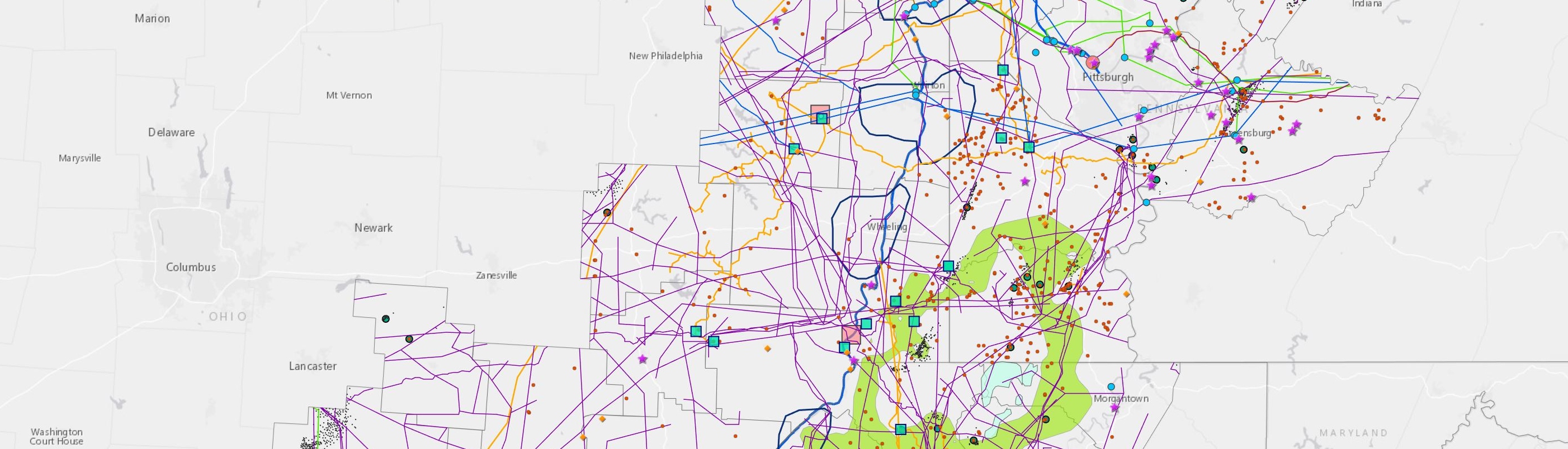
Figure 3. PA Earthquakes and Potential Causes: 1/2000 – 2/2021, Magnitude 2.0 or Greater. Most earthquakes in the eastern portion of the state are associated with Quaternary faults. In the western portion, the causes are less straightforward, and include zipper fracking, mine blasting or collapse, and faults that are more ancient and deeper than the Quaternary faults, many of which remain unmapped. As the use of SWD wells increases, seismic activity may increase as well.
Manmade earthquakes are not limited to Oklahoma. For example, there were approximately 130 seismic events in one year period in the Youngstown, Ohio area due to SWD activity, including one measuring 4.0 on the last day of 2011. Over the years, the regulatory reaction to induced earthquakes seems to walking along the slippery slope from “that can’t happen” to “that can’t happen here” to “they’re all small earthquakes” to “we can mitigate the impact,” despite all evidence to the contrary.
Two Regulators
So who gets to be in charge of this dumpster fire? As mentioned above, this is ultimately under the umbrella of EPA’s Underground Injection Control program. However, they have a complicated arrangement with the various states defining who has primary enforcement authority for this type of well.
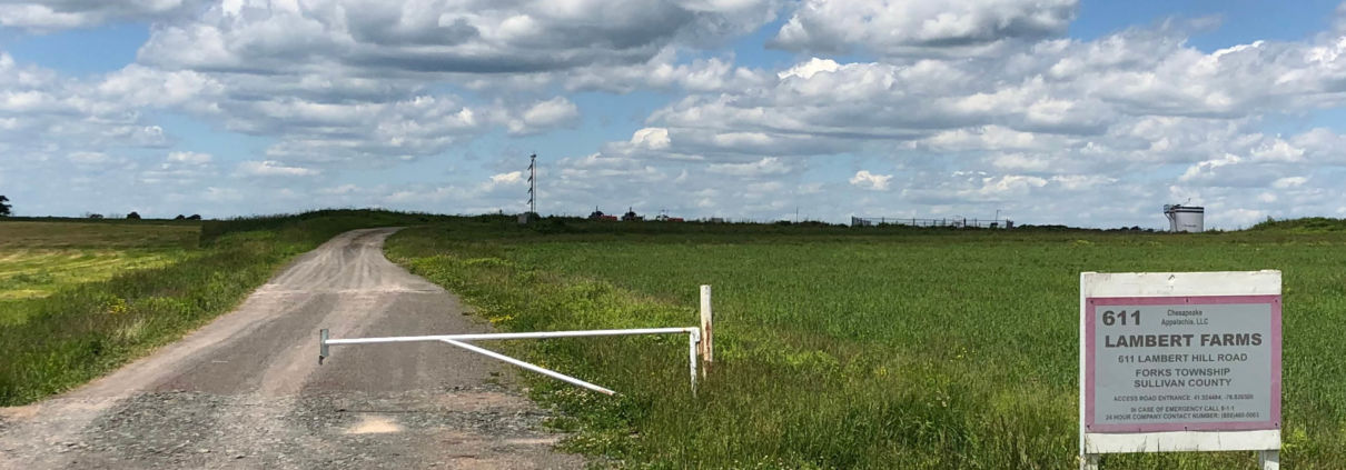
In Pennsylvania, such wells must obtain a permit from EPA before obtaining a second permit from DEP. In a 2017 hearing in Plum Borough, Allegheny County, furious residents concerned with a variety of issues with a proposed SWD well were told that in Pennsylvania, EPA could only consider whether or not the well would violate the 1972 Clean Water Act when considering the permit, and that the correct audience for everything else would be DEP. Both permits for this well that is near and undear to me were ultimately issued, and operations are expected to begin in the next month if Governor Wolf does not instruct the DEP to reconsider their permit.
There is some precedent for overturning such a permit. In March of 2020, DEP yanked a permit for a SWD well in Grant Township, Indiana County, suddenly respecting a home-rule charter law that the agency had previously sued the Township over.
Without the prospect of royalties or impact fees, no community wants these wells and regulators know that they are nothing but problems. However, the reality is that the regulators oversee an industry that produces a tsunami of this toxic waste – more than 61.8 million barrels of it from unconventional wells in Pennsylvania in 2020 according to self-reported data, which is almost 2.6 billion gallons of the stuff, or slightly more than the capacity of Beaverdam Run Reservoir in Cambria County, a 382 acre lake with an average depth of 20 feet.
Unsuitable Geography
Nationally, injection wells are quite common, with over 740,000 such wells in the EPA inventory for 2018 and Class II (O&G) wells represent about a quarter of this figure. Of these Class II injection wells, roughly 20% are for fluid disposal, giving us an estimated 37,000 SWD wells nationwide. This number is expected to go up, as more than three-quarters of the 8,600 permits issued in 2018 were for oil and gas purposes.
However, in Pennsylvania, there have been quite few of these, compared to other states. The primary reason for this is its geology, which has largely been considered unsuitable for this type of activity. For example, a 2009 industry analysis states:
“The disposal of flowback and produced water is an evolving process in the Appalachians. The volumes of water that are being produced as flowback water are likely to require a number of options for disposal that may include municipal or industrial water treatment facilities (primarily in Pennsylvania), Class II injection wells [SWDs], and on-site recycling for use in subsequent fracturing jobs. In most shale gas plays, underground injection has historically been preferred. In the Marcellus play, this option is expected to be limited, as there are few areas where suitable injection zones are available.”
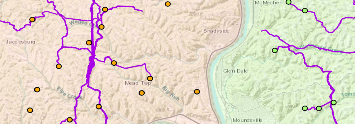
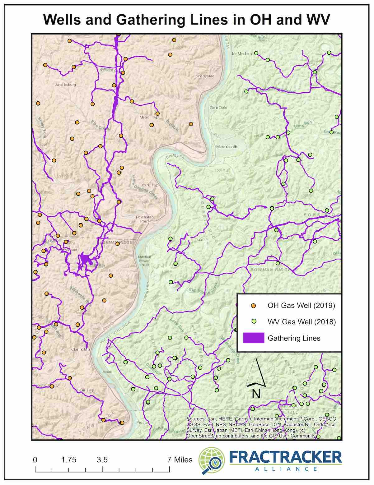
I discussed this topic in a phone call with an official from EPA, who largely confirmed this point of view, but preferred the phrase, “the geology is complicated” instead of the word “unsuitable.” When the UIC program was established from the 1974 Safe Drinking Water Act, there were only seven such wells in operation, and according to EPA’s data, there were still just 11 active SWD wells in the Commonwealth but with more on the way. I was cautioned that the geology wasn’t the only reason, however. Neighboring Ohio had hundreds of these wells, many of which are clustered close to the border with Pennsylvania. The two states have different primacy and permitting arrangements, which is a factor as well.
I have not come across sources mentioning why Pennsylvania’s geology was so unsuitable – or complicated, if we are being generous. However, there are numerous widespread issues that could be a factor, including voids created by karst and legacy coal mines, and formations that might have otherwise trapped gasses and fluids being punctured with up to 760,000 mostly unplugged oil and gas wells and more than one million drinking water wells.
Even when these fluids have been pumped deep underground, they are not necessarily out of sight and out of mind. For example, an abandoned well in Noble County Ohio suddenly began spewing gas field brine just a few weeks ago, resulting in a fish kill in a nearby stream. The incident is believed to be related to SWD wells in the general vicinity even though the closest of these is miles away from the toxic geyser. The waste fluids injected beneath the surface will exploit any pathway available through crumbling or porous rocks to alleviate the pressure built up from the injection process. These fluids don’t care whether the target is an old gas well, mine void, or drinking water aquifer.
Of course, we could ask the question in reverse, and ask what makes the injection of oil and gas fluids suitable in other locations, and the aggregated evidence would lead us to “nothing” as our answer. Nothing, other than the fact that drilling and fracking produces billions of gallons of liquid waste, and that it has to go somewhere.
Although EPA play a major role in permitting and regulating SWD wells in Pennsylvania, they do not publish data related to these wells on their website. FracTracker started hearing rumors about a spate of new SWD permits all over the state that were not accounted for in DEP data. As it turns out, many of these turned out to be other oil and gas wastewater processing facilities, and the public’s confusion about these is completely understandable because these facilities lacked the proper public notice process. These facilities are concerning in their own right – and residents of Pennsylvania should look here to see if one of these 49 facilities are in their neighborhoods – but these are not disposal wells.
To clear up the confusion, I submitted a Freedom of Information Act request to EPA for a spreadsheet of their Class II injection wells in Pennsylvania. This was apparently an onerous task that would require more than ten hours of labor on their behalf. When I mentioned that I was mostly interested in disposal wells, that sped the process up considerably.
Ultimately, I received a portion of the data fields that I had asked for.
Asked For
Received
Well Name
Yes
Well API Number
Yes
Class II Category (disposal, recovery, storage)
No
Date application received
No
Application status (e.g., pending, complete)
Yes
Application result (e.g., approved, rejected)
No
Application result date (date of EPA’s decision)
No
Well status (e.g., active, plugged)
Yes
Well county name
Yes
Well municipality name
No
Well latitude
Yes
Well longitude
Yes
Table 1 – Summary of fields requested and received in FracTracker’s FOIA submission with EPA.
I started to compare the EPA dataset to DEP’s SWD well dataset, which is a part of its conventional well inventory. Each source had 23 records. We were off to a good start, but this data victory turned out to be limited in scope as the discrepancies between the two datasets continued to grow. Inconsistencies between the two datasets are as follows:
County
DEP API
DEP Well Name
EPA API Match
EPA Name Match
Notes
Allegheny
003-21223
SEDAT 3A
Y
Y
Armstrong
005-21675
HARRY L DANDO 1
Y
Y
Beaver
007-20027
COLUMBIA GAS OF PENNA INC CGPA5
Y
Y
Bedford
009-20039
KENNETH A DIEHL D1
N
N
Not on EPA List
Cambria
021-20018
THE PEOPLES NATURAL GAS CO 4627X
N
N
Not on EPA list
Clearfield
033-27255
FRANK & SUSAN ZELMAN 1
N
Y
DEP / EPA API Number mismatch
033-27257
POVLIK 1
N
Y
No EPA API No.
033-00053
IRVIN A-19 FMLY FEE A 19
Y
Y
033-22059
SPENCER LAND CO 2
Y
Y
Elk
047-23835
FEE SENECA RESOURCES WARRANT 3771 38268
Y
Y
047-23885
FEE SENECA RESOURCES WARRANT 3771 38282
N
Y
DEP / EPA API Number mismatch
Erie
049-24388
NORBERT CROSS 2
Y
Y
049-20109
HAMMERMILL PLT 1
N
N
Not on EPA List
049-00013
HAMMERMILL 3
N
N
Not on EPA List
049-00012
HAMMERMILL 1
N
N
Not on EPA List
Greene
N
N
Not on DEP list. EPA Permit PAS2D210BGRE – no API to match
Indiana
063-31807
MARJORIE C YANITY 1025
Y
Y
063-20246
T H YUCKENBERG 1
Y
Y
Somerset
111-20059
W SHANKSVILLE SALT WATER DISP 1
Y
N
111-20006
MORRIS H CRITCHFIELD 1
Y
N
Potter
105-20473
H A HEINRICK RW-55
CA
Y
Category Anomaly – Not on DEP SWD list – does appear as Plugged OG Well (consistent w/ EPA status notes)
Venango
121-44484
LATSHAW 9
Y
Y
Warren
123-39874
BITTINGER 4
N
Y
API Mismatch (But does match Bittinger #1) Lat/Long match site name
123-33914
JOSEPH BITTINGER 1
N
Y
API Mismatch (But does match Bittinger #4) Lat matches site name, Long slightly off
123-33944
JOSEPH BITTINGER 2
Y
Y
123-33945
JOSEPH BITTINGER 3
CA
Y
Category Anomaly – Not on DEP SWD list – does appear as “Injection”
123-34843
SMITH/RAS UNIT 1
CA
Y
Category Anomaly – Not on DEP SWD list – does appear as “Observation”
123-22665
LEROY STODDARD & FRANK COFFA 1 WELL
N
N
Not on DEP list of all wells. Does appear on eFACTS. No location data
Table 2 – Discrepancies between EPA and DEP data for SWD wells in PA.
Altogether, there was at least one data discrepancy on 17 out of 28 wells (61%) on the combined inventories, and this is allowing for significantly different formatting of the well’s name. The DEP list contained five records that were not on the EPA dataset at all, four records where the well’s API number did not match, three instances where the DEP well type was different from EPA’s listing, two wells with matching API numbers but different well names, two wells that were missing the API number on the EPA list, and one well that was on the EPA list that I have not been able to find in any of DEP’s inventories. These last two wells could not be mapped due to the lack of location data.
It isn’t always possible to know which dataset is erroneous, but the EPA list has several obvious omissions and one instance where the API number and well name are in the wrong columns. The quality of DEP data has improved over the years and appear to have some data controls in place to avoid some of these basic errors. For that reason, I suspect that most of the problems stem from the EPA dataset, and I have used DEP coordinates to map these wells.
Waste Disposal Wells in Pennsylvania
This map contains numerous layers that explore the current state of Class II-D Salt Water Disposal (SWD) injection wells for oil and gas waste in Pennsylvania. View the map “Details” tab below in the top left corner to learn more and access the data, or click on the map to explore the dynamic version of this data.
In the early 1970s, it was recognized that industrial injection of oil and gas waste underground could lead to risks to human health and the environment, so several major protective laws were put in place, including the Clean Water Act of 1972, the Safe Drinking Water Act of 1974, and the Pennsylvania’s 1971 Environmental Rights Amendment. Decades later, it feels like the Pennsylvania Department of Environmental Protection and the United States Environmental Protection Agency don’t take their regulatory responsibilities very seriously when it comes to oil and gas liquid waste disposal wells. While the state does have fewer of this type of well than other states, there are five that are currently under construction, according to the EPA dataset. Many of these, like the Sedat 3A well in Allegheny County, have come after significant community opposition, and many of the residents’ concerns have not been addressed by either agency.
There will undoubtedly be more of these disposal wells proposed in the near future. Residents would do well to hassle their municipalities to update their ordinances for this type of well if they happen to live in a place where such ordinances are possible. Solicitors should be instructed to regularly scour the Pennsylvania Bulletin and be in contact with EPA for the earliest possible notification of a proposed site, so that there is time to respond within the comment periods.
Additionally, the sloppiness of the datasets calls all sorts of questions into play regarding the co-regulation of these wells. In the case of an incident, it’s not even clear that both agencies have the information on hand to even locate the site in the field. Meanwhile, a 61% error rate between the sites name, API number, and status does not inspire confidence that agencies are keeping a close eye on these facilities, to say the least.
Above all, we must all realize that it isn’t safe to assume that someone will let us know when these types of facilities are proposed. Regulators have shown us through their actions that they are thinking far more about the billions of gallons of waste that needs to be disposed of than of the well-being of dozens or even hundreds of neighbors near each toxic dump site.
References & Where to Learn More
Data supporting this article, as well as the static map in Figure 3, can be found here.
FracTracker Pennsylvania articles, maps, and imagery: https://www.fractracker.org/map/us/pennsylvania/
https://www.fractracker.org/a5ej20sjfwe/wp-content/uploads/2021/02/Waste-Disposal-Wells-in-Pennsylvania-feature-scaled.jpg6671500Matt Kelso, BAhttps://www.fractracker.org/a5ej20sjfwe/wp-content/uploads/2025/09/2025-Wordmark-Logo.pngMatt Kelso, BA2021-02-26 12:23:392021-04-15 14:08:41Pennsylvania’s Waste Disposal Wells – A Tale of Two Datasets
Kyle Ferrar, Western Program Coordinator for FracTracker Alliance, contributed to the December 2020 memo, “Recommendations to CalGEM for Assessing the Economic Value of Social Benefits from a 2,500’ Buffer Zone Between Oil & Gas Extraction Activities and Nearby Communities.”
The purpose of this memo is to recommend guidelines to CalGEM for evaluating the economic value of the social benefits and costs to people and the environment in requiring a 2,500 foot setback for oil and gas drilling (OGD) activities. The 2,500’ setback distance should be considered a minimum required setback. The extensive technical literature, which we reference below, analyzes health benefits to populations when they live much farther away than 2,500’, such as 1km to 5km, but 2,500’ is a minimal setback in much of the literature. Economic analyses of the benefits and costs of setbacks should follow the technical literature and consider setbacks beyond 2,500’ also.
The social benefits and costs derive primarily from reducing the negative impacts of OGD pollution of soil, water, and air on the well-being of nearby communities. The impacts include a long list of health conditions that are known to result from hazardous exposures in the vulnerable populations living nearby. The benefits and costs to the OGD industry of implementing a setback are more limited under the assumption that the proposed setback will not impact total production of oil and gas.
The comment letter submitted by Voices in Solidarity against Oil in Neighborhoods (VISIÓN) on November 30, 2020 lays out an inclusive approach to assessing the health and safety consequences to the communities living near oil and gas extraction activities. This memo addresses how CalGEM might analyze the economic value of the net social benefits from reducing the pollution suffered by nearby communities. In doing so, this memo provides detailed recommendations on one part of the broader holistic evaluation that CalGEM must use in deciding the setback rule.
This memo consists of two parts. The first part documents factors that CalGEM should take into account when evaluating the economic benefits and costs of the forthcoming proposed rule. These include factors like the adverse health impacts of pollution from OGD, the hazards causing them and their sources, and the way they manifest into social and economic costs. It also describes populations that are particularly vulnerable to pollution and its effects as well as geographic factors that impact outcomes.
The second part of this memo documents the direct and indirect economic benefits of the proposed rule. Here, the memo discusses the methods and data that should be leveraged to analyze economic benefits of reducing exposure to OGD pollution through setbacks. This includes the health benefits, impacts on worker productivity, opportunity costs of OGD activity within the proposed setback, and the fact that impacted communities are paying the external costs of OGD.
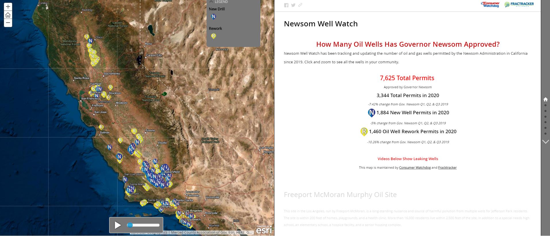
The fossil fuel industry has historically taken advantage of the nation’s mineral estate for private profit, while outsourcing the public health debts of degraded environmental quality to Frontline Communities. While President Biden has recently ordered the Department of Interior to put a 60-day halt on permitting new oil and gas drilling permits on federal lands, no such policy exists for state lands in California. Governor Newsom’s administration has allowed the California Geological Energy Management Division to issue rework and new drilling permits on California state lands, bringing the total number of operational oil and gas wells on state lands up to a total of 178, almost half of which are “idle.” This number pales in comparison to the number of California oil and gas wells on federal lands; a total of 6,997 operational wells.
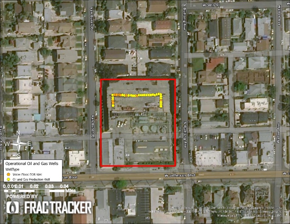
FracTracker Alliance has mapped out the operational oil and gas wells located on state lands in California, using the California Protected Areas Database. The areas containing the highest concentrations of oil and gas wells on state lands include two sensitive ecosystem environments. Figure 1 shows the 102 operational oil and gas wells located in Southern California’s Bolsa Chica Ecological Preserve. The wells are part of the Huntington Beach oil field. The preserve shares marine habitat with a marine protected area (MPA) and is habitat for numerous rare and several endangered species. More sensitive habitat also threatened by oil and gas extraction; Figure 2 shows the oil and gas production wells on the Sacramento River Delta, just upriver of the Bay Area. It is habitat for several threatened and endangered species such as the Delta Smelt and Giant Garter Snake.
California needs Governor Newsom to take a stand against the further exploitation of California’s public lands. A ban on permitting new wells on state land and a commitment to plug existing wells would set an example for Biden’s administration to make the current 60-day freeze a permanent policy.
Figure 1. The Bolsa Chica Ecological Preserve hosts over 100 operational oil and gas wells that put the preserve’s ecological habitat at risk.
Figure 2. There are 50 operational oil and gas wells permitted on California state lands in the Sacramento River Delta.
https://www.fractracker.org/a5ej20sjfwe/wp-content/uploads/2021/02/Figure-2.-There-are-50-operational-oil-and-gas-wells-permitted-on-California-state-lands-in-the-Sacramento-River-Delta-feature-scaled.jpg6671500Kyle Ferrar, MPHhttps://www.fractracker.org/a5ej20sjfwe/wp-content/uploads/2025/09/2025-Wordmark-Logo.pngKyle Ferrar, MPH2021-02-12 17:42:002021-04-15 14:08:43Oil and Gas Wells on California State Lands
Southwest Detroit and neighboring South Rockwood in Monroe County could not be more different demographically, but one thing they have in common is a consistent battle with the extractives industry.
With environmental advocates Theresa Landrum and Doug Wood, FracTracker created a Story Map to document what this infrastructural buildout in Southeastern Michigan looks like from the air, how it has displaced entire neighborhoods, and how it has forever changed their quality of life, in the name of short-term profiteering.
“Marathon is a prime example of corporate polluters continuing
to choose profit over safeguards for our public health.”
– Congresswoman Rashida Tlaib
Each year, FracTracker Alliance gives out its Community Sentinel Award for Environmental Stewardship. We had an amazing group of candidates this year, and the four winners are extremely brave, persistent, insightful, and collaborative activists representing diverse communities all over the country.
I have had the good fortune to interact with two of the winners – Theresa Landrum and Brenda Jo McManama – quite frequently over my time at FracTracker. This year’s Sentinel Award winners and all its previous recipients are passionate and persistent fighters for environmental justice in their own backyards and around the United States.
It is around this time of year that all the negativity involved in the fight against fossil fuel industries dissolves away for me as I find myself inspired and humbled by the Sentinel winners. Theresa and Brenda Jo constantly inspire me and FracTracker to strive to do more, do better, and remain cleareyed as to whom we serve. All the Community Sentinel nominees are exemplars of what it is to walk authentically and humbly through life.
However, I am going to spend the next couple paragraphs speaking specifically about Ms. Landrum, because it is she that I have come to know and work quite well with since COVID-19 was something we thought would be gone by June.
I had heard so many amazing things about Ms. Landrum from a common comrade, Mr. Doug Wood, whom FracTracker has written about with respect to the silica sand mining he is fighting and dubious pro-mining legislation being pushed in Michigan’s Statehouse, but I had never met her in person. That changed on a scorching hot day this past June, when Doug, Theresa, and I met (socially distanced) in the shadow of Marathon Petroleum’s refinery at Detroit’s Kemeny Recreation Center, just a couple stones throws across I-75 (see images below).
“Marathon is a prime example of corporate polluters continuing to choose profit over safeguards for our public health. It is time to say enough is enough of Marathon’s constant disregard of the health and safety of residents who live, work, and visit the surrounding communities. Marathon has perpetrated numerous incidents detrimental to our communities and must be held accountable – they clearly cannot be trusted to protect our health. I look forward to discussing the need to hold Marathon and other entities who poison our community accountable and solutions to make our communities breathe and live free at the upcoming congressional field hearing I am hosting with other members of Congress, experts, and grassroots activists here in Detroit.”
Southeastern Michigan Environmental Activists Doug Wood and Theresa Landrum at Detroit’s 48217 Kimeny Park with Marathon’s Refinery in the Background, June, 2020
Anti-Frac Sand mine signage created by Monroe County, Michigan activist Doug Wood, June, 2020
No Dumping signage erected by Marathon Oil in Detroit’s Oakwood Neighborhood adjacent to the company’s oil refinery
Concerned Citizen and Sylvania Minerals mine neighbor Doug Wood
It did not take more than 30 seconds for me to realize that Theresa was an authentic and persistent fighter for her community, and that she belongs on the Mt. Rushmore of EJ advocates – as does Doug Wood and all of the Community Sentinel nominees past, present, and future.
After meeting at the recreation center, I followed Theresa around with my drone, capturing footage and images of the worst actors in the 48217 zip code of Southwest Detroit, as well as of River Rouge and Ecorse. This turned out to be the first of three trips to meet with Theresa throughout the summer and fall of 2020.
During each trip and across dozens of phone conversations, Theresa explained to me what industry has done to Southwest Detroit, how she has gone about combatting it, and the way that Lansing treats Wayne County.
It struck me that much of her experience overlaps with the stories I have heard in disparate demographics, from soybean farmers in LaSalle County, Illinois, to dairy farmers in Western Wisconsin, all the way to coalminers in Central Appalachia.
Their stories illustrate the near universal tale of how industry needs and welfare demands take precedence over the rights of citizens. It is the story of globalization, shareholder returns, and political/economic elites ignoring, mocking, or being deaf and blind to the needs of their constituents and the crimes being committed in the name of progress and Gross Domestic Product (GDP).
One thing Theresa and I have spent quite a bit of time discussing is the overlap in environmental justice across demographics, and how superficial differences have been weaponized to divide us, leaving only corporations and their political handmaids to benefit. Industry beneficiaries and politicians have colluded to declare in the words of Thomas Frank’s latest book “The People, No!” Yet, it is people like Theresa, Doug, Brenda Jo, and all the other environmental activists we celebrate who are and will be instrumental in bridging those divides, and guiding the citizenry to pivot, to identify and defeat the real Leviathan – the Hydrocarbon Industrial Complex in all its manifestations and with all its tentacles spread out across this country.
The best way I know how to return the favor to folks like Theresa is to continue to do what FracTracker does best, and what I hope I am doing well, which is documenting the infrastructure and landscapes that are or have been in the crosshairs of industry, whether it be steel, coal, oil, or in the case of our name – fracked natural gas.
I have been working with Theresa and Doug on a Story Map that illustrates the scale and scope of industrial impacts in southeastern Michigan, from US Steel’s Zug Island to Sylvanian Mineral’s frac sand mine in South Rockwood. As I mentioned above, we have outlined the plight of Doug and Dawn Wood in their fight against their neighbor Sylvanian Minerals. However, with respect to Southwest Detroit, it is critical that we give a bit of background to the region’s cultural significance. For that, I am going to refer to Ms. Landrum’s own words, shared below:
A Historical Perspective of Wayne County Michigan’s Tri-Cities Region
By Theresa Landrum
During the first and second waves of the early 20th Century Great Migration, African Americans came from the South to Michigan’s communities of Ecorse (48229), River Rouge (48218), and Southwest Detroit (48217), AKA the “Triple Cities,” seeking factory jobs in the surrounding industries; U.S. Steel (formerly Great Lakes Steel), Ford Motor Company, Zug Island, Dana Corporation, and BASF Chemicals. During this time, many white men enlisted in the armed forces, and employers needed workers – so companies recruited southern African Americans to fill the jobs.
This region is one of the first African American settlements in Michigan after World War II, where Black people could actually buy homes, which helped establish metro Detroit’s Black middle class.
By the 1930s and 40s it was a self-sustaining area rich with opportunities, a mecca for Black-owned businesses, like gas stations, stores, jazz clubs, restaurants, hotels, laundromats, dry cleaners, and much more. It was also the home of Black professionals: doctors, pharmacists, policemen, florists, bakers, dentists, teachers, lawyers, and realtors thrived here, and was the site of one of Michigan’s first Black hospitals, Sidney A. Sumby Memorial Hospital, built by Black doctors.
The thread that ties these three communities/zip codes together is their formation of (what was then) Ecorse Township. Their division came after the City of Detroit expressed interest in annexing the River Rouge area. River Rouge incorporated into a village to ward this off, but Detroit was able to annex the Southwest 48217 area in 1922, thus segmenting Ecorse Township into three parts.
Fast forward to the 1950s, when Detroit’s landscape changed forever with the government’s declaration of “Eminent Domain” that claimed many African American homes for construction of the I-75 Expressway, which runs right through the center of Southwest Detroit’s (SWD) 48217 community. As I-75 was constructed, Ohio Oil (which officially became Marathon Oil in 1962) also increased its footprint in the area by acquiring nearly 100 acres and destroying a wetland habitat to expand its storage tank farm, which to date has over 100 storage tanks.
Marathon expanded again in 2007 with the announcement of the $2.2 billion Detroit Heavy Upgrade Project (DHOUP), where they would transition to refining dirty tar-sands from Alberta, Canada. This increased production to 120,000 barrels of crude per day, and thus increased the expulsion of harmful, pollutive emissions into the nearby neighborhoods. The project was completed in 2012, which also resulted in Marathon buying over 400 homes in the SWD 48217 (Oakwood Heights) area, further encroaching into residential communities.
Theresa was a recipient of the 2020 Community Sentinel Award for Environmental Stewardship, presented by FracTracker Alliance and Halt the Harm Network. Read more about her story here.
The Thoughts of Dawn & Doug Wood About Living Next to a Frac Sand Mine
I asked Dawn and Doug Wood to send me their thoughts on what it is like living next to Sylvanian Minerals and US Silica’s frac sand mine in South Rockwood, Michigan. I extracted (and clarified where necessary) the excerpts below that clearly illustrate their frustrations with their community, local, and federally elected officials, as well as the mine operators:
“[The] list of insurmountable mini-nightmares of living next to a frac sand mine [is endless at this point]. [Ten] years ago, they wanted to annex this quarry. [Our] village government has exercised no control over this corporation. [T]he village and the quarry refuse to do any air monitoring, [and] the residents who voted [in favor of] this quarry continue to be silent against any controls over this quarry. Residents seem to fear retaliation if they speak out against [the] village/quarry, [and to this day we] can’t quite explain the community’s lack of outrage … [We] have been shaking our head for years about this … It’s like the pandemic, it is invisible, yet it is killing people … [and] we are living in a polluted community, so our lungs are already taxed [which amplified the impacts of COVID]. [We] have been petitioning for air monitors and dust controls for four years, [and to add insult to injury] after ten years of this bull- – – -, the industry proposes Senate Bill 431 to totally strip communities of their controls, allowing mines to expand whenever they want, and new quarries to just be approved wherever they want [which has prompted the industry to correctly assume] they are entitled. PURE MICHIGAN is the state slogan. We think that’s PURE BULL- – – -!!”
A Southwestern Detroit and Neighboring Monroe County Industrial Impacts Story Map
Southwest Detroit and neighboring South Rockwood in Monroe County could not be more different demographically, but one thing they have in common is a consistent battle with the extractives industry.
We built this Story Map to identify the industrial bad actors and census-level indicators such as mean annual income, and most importantly, to present a growing library of georeferenced drone footage and imagery we have collected over the years.
There have been dozens of other industrial projects foisted on the Triple Cities area of Detroit during this period and to the present day. The goal of this Story Map was to document with drone photography what this infrastructural buildout looks like from the air, how it has displaced and been incorporated directly into neighborhoods – and in the case of Sylvanian Mineral’s South Rockwood facility operating adjacent to good people like the Woods – how it has forever changed their quality of life, in the name of short-term profiteering.
We will continue to “infill” and expand this Story Map in the coming months and years, especially throughout greater Wayne County and the surrounding counties, as southeastern Michigan continues to act as a chokepoint for all manner of industrial and fossil fuel operators and activities. Furthermore, this collaborative effort with Ms. Landrum demands her community’s involvement and acceptance. We also strive to make this project a valuable resource for Michigan-based environmental NGOs and the state’s excellent journalists, like Steve Neavling at Detroit MetroTimes, and Evan Kutz at Great Lakes Beacon.
We plan to update this Map with more culturally significant imagery from the Detroit Public Library and The Wayne State Walter Reuther Library to include media focusing on labor strife, police violence, and the rich tradition and history of the region’s artistic heritage. Additionally, we will expand the depth and breadth of our drone imagery library, as well as continue our nascent effort to collect the stories of regional elders who speak to Southwest Detroit as one of the fulcrums of African American culture, and who explore how industrial colonialism has decimated much the area’s sense of place and community pride.
However, I am confident and hopeful that with progressive voices like Congresswoman Tlaib, committed journalists like those previously mentioned, and activists like Ms. Landrum passing the torch to a younger generation of activists, Southwest Detroit’s condition will take a turn for the better.
Footnote on Michigan’s Senate Bill 431
We wrote about the impacts that SB 431 would have on Michigan’s community and ecosystems last summer, when we were outlining some of the industry’s efforts in Statehouses across the country to weaken environmental regulations – and in some cases, the democratic process itself. SB 431, in particular, would have made the process of operating a sand and gravel mine in Michigan much easier, by way of removing local participation. As the Metamora Land Preservation Alliance (MLPA) wrote in opposition to the bill, this legislation would have allowed for “uncontrolled gravel mining” throughout the state. However, in a bit of good news, a large coalition of Michigan environmental organizations was able to defeat this bill with the MLPA, writing the following on its Facebook page:
“KILLER GRAVEL BILLS DEFEATED!!!
SENATE BILLS 431/849 DEFEATED!
NO SENATE VOTE THIS YEAR – BILLS ARE DEAD!
After almost 18 months of battling in Lansing – Senate Bills 431 & 849 (sponsored by Senator Hollier (D) Detroit) – have been defeated. They will not be coming up for a vote this calendar year, and by Senate rules they will therefore expire. Thus ending, for this year, the dire threat of uncontrolled gravel mining, endangerment of our groundwater, and loss of control of how our communities grow and develop. Make no mistake – this was a serious threat to Michigan’s citizens and communities – and it was a no-holds-barred fight in Lansing.”
Wins for communities over corporations like this are rare, indeed, and should be celebrated. Congratulations to the Woods, MLPA, and all the Michigan communities and organizations that pushed back against this bill. You are true Community Sentinels!
Theresa Landrum, of Detroit, Michigan, 48217. The Original United Citizens of Southwest Detroit; 48217 Community and Environmental Health Organization; Michigan Advisory Council on Environmental Justice; Sierra Club Detroit Chapter, MEJC Clean Air Council; Michigan PFAS action response team
This report focuses on the two immediate stakeholders impacted by oil and gas well drilling setbacks: Frontline Communities and oil and gas operators. First, using U.S. Census data this report helps to define the Frontline Communities most impacted by oil and gas extraction. Then, using GIS techniques and California state data, this report estimates the potential impact of a setback on California’s oil production. Results and conclusions of these analyses are outlined below.
Previous statewide and regional analyses on proximity of oil and gas extraction to various demographics, including analyses included in Kern County’s 2020 draft EIR, have inadequately investigated disparate impacts, and have published erroneous results.
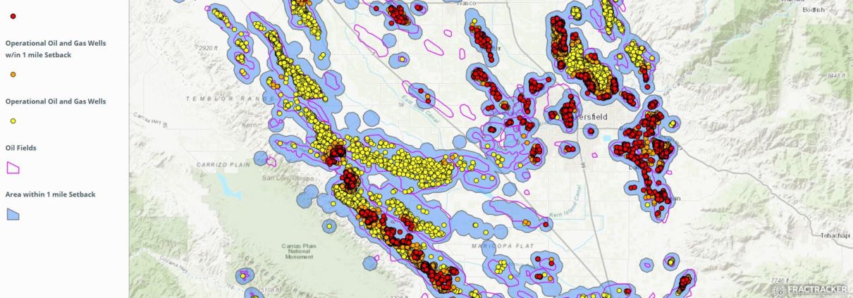
This analysis shows that approximately 2.17 million Californians live within 2,500’ of an operational oil and gas well, and about 7.37 million Californians live within 1 mile.
California’s Frontline Communities living closest to oil and gas extraction sites with high densities of wells are predominantly low income households with non-white and Latinx demographics.
The majority of oil and gas wells are located in environmental justice communities most impacted by contaminated groundwater and air quality degradation resulting from oil and gas extraction, with high risks of low-birth weight pregnancy outcomes.
Adequate Setbacks for permitting new oil and gas wells will reduce health risks for Frontline Communities.
Setbacks for permitting new oil and gas wells will not decrease existing California oil and gas production.
Phasing out wells within setback distances will further decrease health risks for Frontline Communities.
Phasing out wells by disallowing rework permits within a 2,500’ setback distance will have a minimal impact on overall statewide oil production, estimated at an annual maximum loss of 1% by volume.
Setbacks greater than 2,500’ in combination with other public health interventions are necessary to reduce risk for Frontline Communities.
Based on the peer reviewed literature, a setback of at least one mile is recommended.
The energy focused on instituting policies to protect the health of Frontline Communities in California from the negative impacts of oil and gas extraction is at an all-time high. In August 2020, Assembly Bill 345 was heard in the State Senate’s Natural Resources Committee, but was blocked from reaching the Senate floor for a vote. The bill would have required the Geologic Energy Management Division in the Department of Conservation (CalGEM) to establish a minimum setback distance between oil and gas production and related activities and sensitive receptors like homes, schools, and hospitals. While this strong effort to establish health and safety setbacks through the state legislature may have failed, the movement has paved the way for local actions. Additionally, California is in the midst of a statewide public health rule-making process to address the health impacts of oil and gas extraction currently experienced by Frontline Communities.
In related advocacy, Frontline Community groups in California recommended a minimum 2500’ setback based on scientific studies, including a 2015 report by the California Council on Science and Technology which identified “significant” health risks at a distance of one-half mile from drill sites. A recent grand jury report from Pennsylvania recommended 5,000’ setbacks, with 2,500’ as a minimum requirement to address the most impacted communities. Additionally, the state of Colorado has recently adopted 2,000’ setbacks for homes and schools, while the existing 2,000’ setback has had minimal impacts on oil and gas production.
In September 2020, Governor Newsom declared the deadline for the first draft of the pre-regulatory rule-making report will be the first of January 2021. FracTracker Alliance has therefore completed an updated assessment of the Frontline Communities most impacted by oil and has projected the potential impact on oil and gas extraction operations. An interactive map of oil and gas activity and Frontline Communities is shown below in Figure 1. The map identifies the operational (active, idle, and new) oil and gas wells located within 2,500’ and 1 mile buffer zones from sensitive receptors, defined as homes, schools, licensed daycares and healthcare facilities.
The impacts of oil and gas drilling do not stop at 2,500’, as regional groundwater contamination and air quality degradation of ozone creation and PM2.5 concentrations are widespread hazards of oil and gas extraction. Phasing out wells within 2,500’ of homes will reduce the negative health effects for the Frontline Communities bearing the brunt of the risks associated with living near oil and gas wells, as well as reduce regional environmental hazards. These risks include over 24 categories of health impacts and symptoms associated with 14 bodily systems, including eyes, ears, nose, and throat; mental health; reproduction and pregnancy; endocrine; respiratory; cardiovascular and pulmonary; blood and immune system; kidneys and urinary system; general health; sexual health; and physical health among others. The most regularly documented health outcomes include mortality, asthma and respiratory outcomes, cancer risk including hematological (blood) cancer, preterm birth, low birth weight and other negative birth outcomes.
The interactive map below in Figure 1 shows the operational oil and gas wells located within 2,500’ of sensitive receptors, including homes, schools, healthcare facilities, prisons, and permitted daycares. Overall in the state of California, 16,724 operational (8,618 active, 7,786 idle, and 320 new) wells are located within the 2,500’ setback. Of the total ~105,000 operational (62,000 active, 37,400 idle, and 6,000 new), about 16% are within the setback. These wells accounted for 12.8% of the total oil/condensate produced in California in 2019. Table 1 below shows the counties where these wells are located, by well permit status. It bears noting that these figures on well location and production represent only a snapshot of current industry activity. As discussed below, current setback proposals would provide a phase out period for existing wells that would greatly reduce any immediate impact on production. Further, directional and even horizontal drilling is common in California, meaning operators can relocate their surface drilling equipment to safer distances and still access oil and gas reserves to maintain production.
Table 1. Status of wells within the 2,500’ setback zone, by county. The table shows the counts of wells located within the 2,500’ setback from homes and other sensitive receptors, broken out by the status of the wells.
Figure 1. Map of California operational oil and gas wells with 2,500’ and one mile setback distances. One mile setbacks are included as a minimum recommendation of this report based on peer reviewed literature. This report recommends the state of California consider one mile as a minimum setback distance to protect Frontline Communities. As you zoom into the map additional, more detailed layers will appear.
Methods (Quick Overview)
In this article we conducted spatial analyses using both the demographics of Frontline Communities and the amount of oil produced from wells near Frontline Communities. This assessment used CalGEM data (updated 10/1/20) to map the locations of operational oil and gas wells and permits, as shown above in Figure 1. The analyses of oil production data utilized CalGEM’s annual production data reporting barrels of oil/condensate. GIS analyses were completed using ESRI ArcGIs Pro Ver. 2.6.1 with data projected in NAD83 California Teale Albers.
Wells within 2,500’ and 1 mile of sensitive receptors were determined using GIS techniques. This report defines sensitive receptors as residences, schools, licensed child daycare centers, healthcare facilities. Sensitive receptor datasets were downloaded from California Health and Human Services, and the California Department of Education.
We used block group level “census designated areas” from American Community Survey (2013-2018) demographics to estimate counts of Californians living near oil and gas extraction activity. Census block groups were clipped using the buffered datasets of operational oil and gas wells. A uniform population distribution within the census blocks was assumed in order to determine the population counts of block groups within 2,500’ of an operational oil and gas well, 2,500’ to 1 mile from an operational well, and beyond 1 mile from an operational well. Census demographics and total population counts were scaled using the proportion of the clipped block groups within the setback area (Areal percentage = Area of block group within [2,500’; 2,500’-1 mile; Beyond 1 mile] of an operational well / Total area of block group).
This conservative approach provided a general overview of the count and demographics of Californians living near extraction operations, but does little to shed light on most impacted Frontline Communities; specifically urban areas with dense populations near large oil fields. More granular analyses at the local level were necessary to address the spatial bias resulting from non-uniform census block group dimensions and population density distributions, as well as the distribution of operational oil and gas wells within the census block groups. Consequently, we conducted further analysis utilizing customized sample areas for each oil field, which were selected manually using remote sensing data. Full census blocks were used to summarize the actual areas and the urban populations constituting the majority of Frontline Communities.
In the localized, static maps that follow, the census blocks included in the population summaries are shown in pink, while the surrounding census blocks are shown in blue. As seen in Table 2, census data for this initial environmental justice assessment was limited to “Race” (Census Table XO2), “Hispanic or Latino Origin” (Census Table XO3) and several other indicators including “Annual Median Income of Households” (Census Table X19) and “Poverty” (Census Table X17).
Results and Discussion
California Statewide Analysis
Demographics
As a baseline, it is important to provide statewide estimations to track the total number of Californians living near oil and gas extraction operations. This analysis showed that about 2.17 million Californians live within 2,500’ of an operational oil and gas well, and about 7.37 million Californians live within 1 mile. The demographics of these communities at and between these distances is shown below in Table 2, alongside demographic estimates of the California population living beyond 1 mile from an oil and gas well. Census block groups closer to oil and gas wells have higher proportions of Non-white (calculated by subtracting “White Only” from “Total Population”) and Latinx (“Hispanic or Latino Origin”) populations, as well as higher proportions of low-income households, based on both median annual income and poverty thresholds. The analysis show that communities living closer to oil and gas wells have higher percentages of non-white and Latinx populations when compared to the population living beyond 1 mile from an operational oil and gas wells. Communities closer to oil and gas wells are also more likely to be closer to the poverty threshold with lower median annual household incomes.
Table 2. The table shows statewide demographics at multiple distances from operational oil and gas wells. Included are estimates of the non-white and Latinx proportions of the populations within set distances from operational oil and gas wells. The percentage of populations within several poverty thresholds were also summarized, along with median annual household income and age.
CalEnviroScreen data, like U.S. Census data, is also aggregated at the census block group level. While this data can also suffer from the same spatial bias as the statewide analysis above, CES is still very useful to visualize and map the regional pollution burden to assess disparate impacts. The results of the analysis are shown below in Table 3. Counts of operational oil and gas wells for ranges of CES percentile scores. Higher percentiles represent increased environmental degradation or negative health impacts as specified. Of note, the majority of operational oil and gas wells are located in census tracts with the worst scores for air quality degradation and high incidence of low birth weight.
The large number of wells located in the 60-80th percentile rather than the worst (80-100th percentile) is a result of spatial bias, and the many factors that are aggregated to generate the CES Total Scores. These factors include relative affluence and other indicators of socio-economic status. The majority of the worst (80th-100 percentile for Total CES Score) census block groups are located in low-income urban census block groups, many in Northern California cities that do not host urban drilling operations.
This spatial bias results from edge effects of census block groups, where communities living near oil and gas extraction operations may not live in the same census block groups as the oil and gas wells, and are therefore not counted. The authors would recommend future analyses be designed that use CES data to assess disparate impacts in the census block groups most impacted by oil and gas extraction. Neighboring census block groups that do not physically contain operational wells still suffer the consequences of proximity.
For the asthma rankings, the majority of wells are located in the best CES 3.0 percentile (0-20th percentile) for Asthma. While there is much urban drilling in Los Angeles, the spatial bias in this type of analysis gives more weight to the majority of oil and gas wells that are located in rural areas, which historically have much lower asthma rates. This is a result of the very high incidence of asthma in cities without urban drilling such as the Bay Area and Sacramento (80-100th percentile).
Table 3. Counts of operational oil and gas wells in select CalEnviroScreen 3.0 indicators census tracts.
Operational Well Counts by CES3.0 Percentile
0-20%ile
20-40%ile
40-60%ile
60-80%ile
80-100%ile
PM2.5 Air Quality Degradation
5,708
4,237
16,614
7,089
69,987
Ozone Air Quality Degradation
2,238
5,435
6,107
9,898
79,957
Contaminated Drinking Water
1,019
1,675
53,452
6,214
41,206
High Incidence of Low Birth Weight
10,186
13,368
14,995
3,236
58,036
High Incidence of Asthma
40,247
19,827
18,902
4,867
19,792
Total CES 3.0
1,583
5,756
15,671
65,356
12,985
Spatial Bias
Using census data to assess the demographics of those communities most affected by oil and gas drilling can produce misleading results both because of how census designated areas (census tracts and block groups) are designed and because of the uneven distribution of residents within tracts. For example, the majority of Californians who live closest to high concentrations of oil and gas extraction, such as the Kern River oil field, do so in residentially zoned cities and urban settings. In most Frontline Communities the urban census designated areas do not actually contain many wellsites. Instead urban census designated areas are located next to the “estate” and “industrial” (including petroleum extraction) zoned census designated areas that contain the well-sites.
Estate and industrially zoned census designated areas contain the majority of well-sites in Kern County. They are much larger than residentially zoned areas with very low population densities and higher indicators of socioeconomic status. Population centers within the estate zoned areas are often located on the opposite end and farther from well sites than the lower income communities and communities of color living in the neighboring, residentially-zoned census designated areas (e.g., Lost Hills and Shafter). In these cases the statewide demographic summaries above misrepresent the Frontline Communities who are truly closest to extraction operations. Localized environmental justice demographics assessments can also be manipulated in this way.
For instance, The 2020 Kern County draft EIR (chapter 7 PDF pp. 1292-1305) used well counts aggregated by census tracts to conclude that wells in Kern County were not located in disparately impacted communities. Among other requirements for scientific integrity, the draft Kern EIR fails to take into account how the shape, size, and orientation of census designated areas affect the results of an environmental justice assessment. In addition, the EIR uses low-resolution data summarized at the census tract level. Census tracts are much too large to be used to investigate localized health impacts or disparities. Using these blatantly inadequate methods, the draft EIR even claimed Kern County’s oil and gas wells are predominantly located in higher income, white communities, which is outright wrong. For more specific criticisms of the Draft EIR read the FracTracker analysis of the 2020 Kern County EIR.
Results from these types of analyses can be very misleading. Using generalized methods of attributing wells to specific census designated areas does little to identify the communities most impacted by the localized environmental degradation resulting from oil and gas extraction operations, particularly when large census areas such as census tracts are used.
This report therefore takes a different approach, focusing directly on California’s most heavily drilled communities. To understand who and which communities are most harmed by the large-scale industrial oil and gas extraction operations in California, spatial analyses must be refined to focus individually on the communities closest to the highest density extraction operations. For the analyses below, census block groups within 2,500’ of ten different Frontline Communities, all located near some of California’s largest oil and gas fields, were manually identified. The selected block groups’ major population centers were all located within the 2,500’ buffers. Unlike the statewide analysis above, the localized analyses below do not assume homogenous population distributions. Using these methods, FracTracker has identified and demographically described some of the most vulnerable California communities most at risk to the impacts of oil and gas extraction. In the maps below, the “case” census block groups used to generate descriptive demographic summaries of at risk communities bordering extraction operations are outlined in pink, while surrounding census block groups are outlined in light blue.
Well Density
The analyses above are important to understand some of the public health risks of living near oil and gas drilling in California. Yet the methods above used statewide aggregation of well counts and static buffers that do not not show the spectrum of risk resulting from well density. Numerous Frontline Communities in California are within 1 mile or even 2,500’ of literally thousands of oil and gas wells. Conversely, there are many census areas in California that have been included within the spatial analysis of the full state, as described above, located near a single low producing well. Therefore the above methods conservatively summarize demographics and dilute the signal of disparate impacts for low income communities of color. Those methods are not able to differentiate between such scenarios as living near one low-producing well in the Beverly Hills golf course versus living in the middle of the Wilmington Oil Field.
As with any toxin, the dosage determines the intensity of the poison. In environmental sciences, increasing exposure to toxins by increasing the number of sources of a toxin can increase the dosage and therefore the severity of the health impact. The impact of well density has been documented in numerous epidemiological studies as a significant indicator of negative health outcomes, including recently published reports from Stanford University and The University of California – Berkeley linking adverse birth outcomes with living near oil and gas wells in California (Tran et. al 2020, Gonzalez et. al 2020). Therefore the rest of this report focuses on the Frontline Communities living near large oil extraction operations–i.e., oil fields with high densities of operational oil and gas wells.
Kern County
Toggle between the sections below by clicking in the upper left corner of the title bar.
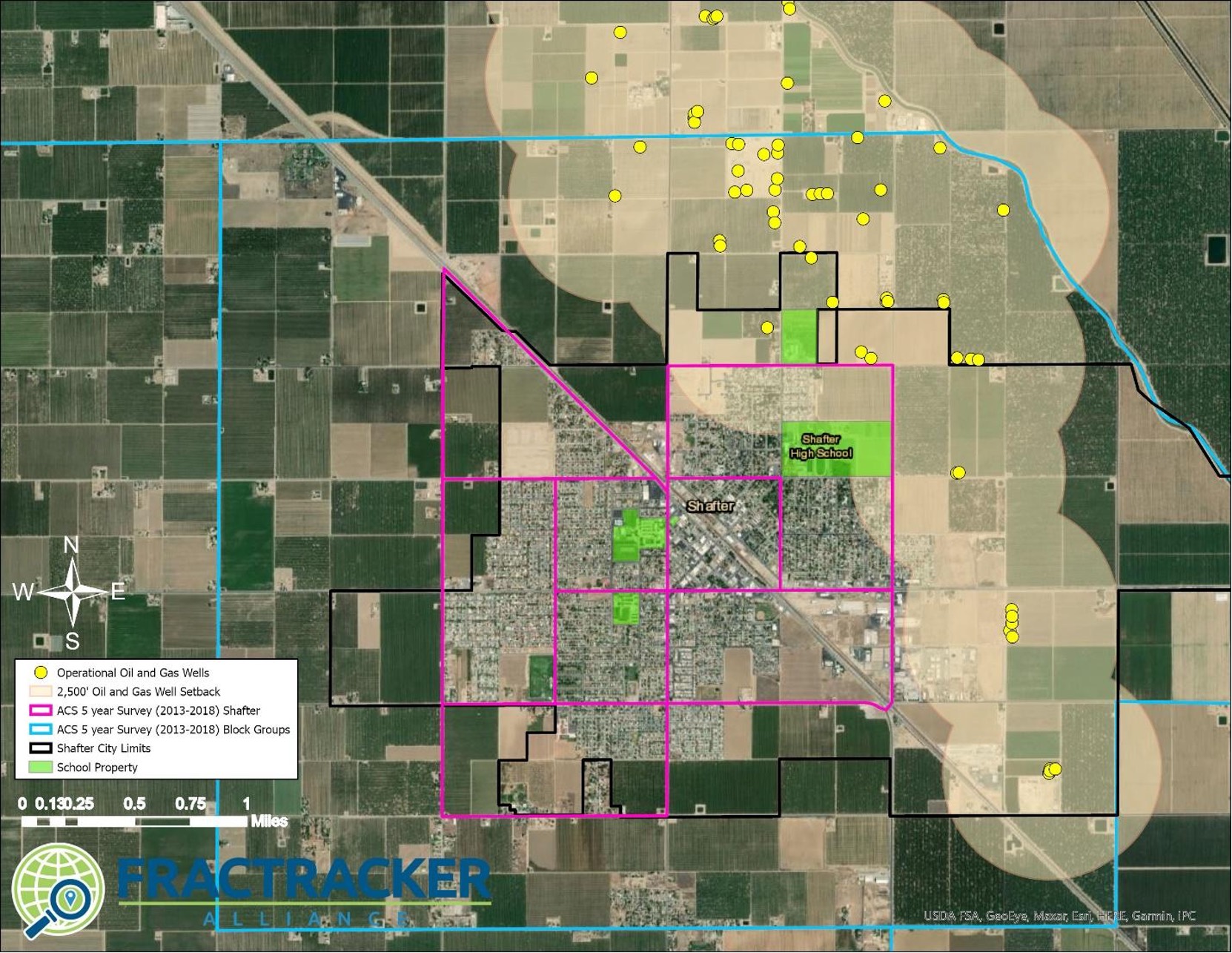
Shafter
The City of Shafter, California, is located near more than 100 operational wells in the North Shafter oil field, as shown below in the map in Figure 2. Technically, the wells are located within a donut-shaped census block group (outlined in blue) that surrounds the limits of the urban census block groups (outlined in pink). Shafter’s population of nearly 20,000 is over 86% Latinx, but the surrounding “donut” with just 2,000 people is about 70% Latinx, much wealthier, and with very low population density. The other neighboring rural census areas housing the rest of the Shafter oil field wells follow this same trend.
An uninformed analysis, such as the Kern County EIR, would conclude that the 2,000 individuals who live within the blue “donut” are at the highest risk, because they share the same census designated area as the wells. Notably, the only population center of this census block group (or census tracts, which follow this same trend) is at the opposite end of the block group, farthest from the Shafter oil field. Instead, the most at-risk community is the urban community of Shafter with high population density; the census block groups within the pink hole of the donut contain the communities and homes nearest the North Shafter field.
Figure 2. The City of Shafter, California is located just to the south of the North Shafter oil field. The map shows the 2,500’ setback distance in tan, as well as the census block groups in both pink and blue. Pink block groups show the urban case populations used to generate the demographic summaries.
Lost Hills, Arvin, & Taft
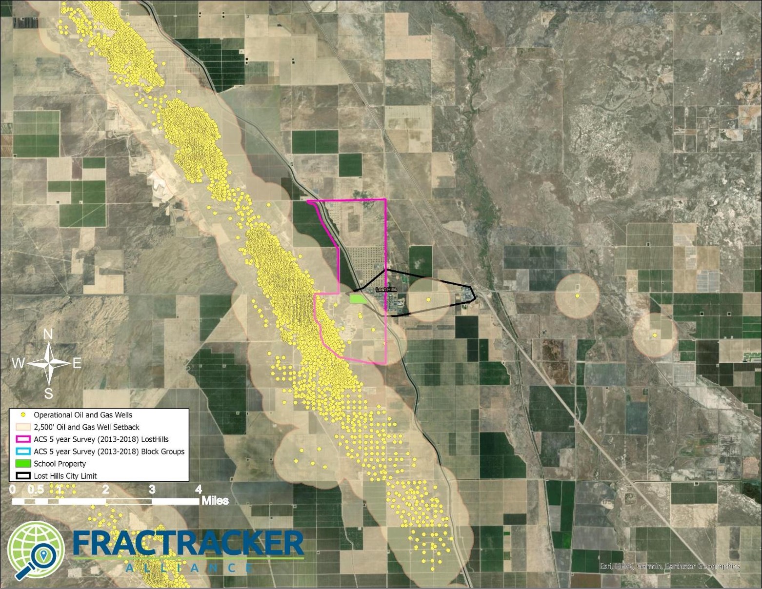
The cities of Lost Hills, Arvin, and Taft are all very similar to Shafter. The cities have densely populated urban centers located within or directly next to an oil field. In the maps below in Figures 3 readers can see the community of Lost Hills next to the Lost Hills oil field. Lost Hills, like the densely populated cities of Arvin and Taft, are located very close to large scale extraction operations. Census block groups that include the most impacted area of Lost Hills is outlined in pink, while surrounding low population density census block groups are shown in blue. The majority of the areas outlined in blue are zoned as “estate” and “agriculture” areas. The outlines of the city boundaries are also shown, along with 2,500’ and 1 mile setback distances from currently operational oil and gas wells.
Lost Hills is another situation where a donut-shaped census area distorts the results of low resolution demographics assessments, such as the one conducted by Kern County in their 2020 Draft EIR (PDF pp. 1292-1305). Almost all of the wells within the Lost Hills oil fields are just outside of a 2,500’ setback, but the incredibly high density of extraction operations results in the combined impact of the sum of these wells on degraded air quality. While stringent setback distances from oil and gas wells are a necessary component of environmental justice, a 2,500’ setback on its own is not enough to reduce exposures and risk for the Frontline Community of Lost Hills. For these Frontline Communities, a setback needs to be much larger to reduce exposures. In fact, limiting a public health intervention to a setback requirement alone is not sufficient to address the environmental health inequities in Lost Hills, Shafter, and other similar communities.
Lost Hill’s nearly 2,000 residents are over 99% Latinx, and over 70% of the households make less than $40,000 in annual income (which is substantially less than the annual median income of Kern County households [at $52,479]). The map in Figure 3 shows that the Lost Hills public elementary school is located within 2,500’ of the Lost Hills oil field and within two miles of more than 2,600 operational wells, in addition to the 6,000 operational wells in the rest of the field.
The City of Arvin has 8 operational oil and gas wells within the city limits, and another 71 operational wells within 2 miles. Arvin, with nearly 22,000 people, is over 90% Latinx, and over 60% of the households make less than $40,000 in annual income.
Additionally the City of Taft, located directly between the Buena Vista and Midway Sunset Fields, has a demographic profile with a Latinx population at least 10% higher than the rest of southern Kern County.
Lost Hills, Arvin, and Taft are among the most impacted densely populated areas of Kern County and represent the most Kern citizens at risk of exposure to air quality degradation from oil and gas extraction.
In all of these cases, if only census tract well counts are considered, like in the 2020 Kern County draft EIR, these Frontline Communities will be completely disregarded. Census tracts are intentionally drawn to separate urban/residential areas from industrial/estate/agricultural areas. The census areas that contain the oil fields are very large and sparsely populated, while neighboring census areas with dense population centers, such as these small cities, are most impacted by the oil and gas fields.
Figure 3. The Unincorporated City of Lost Hills in Kern County, California is located within 2,500’ of the Lost Hills Oil Field. The map shows the 2,500’ setback distance in tan, as well as the census block groups in both pink and blue. Pink block groups show the urban case populations used to generate the demographic summaries.
Bakersfield
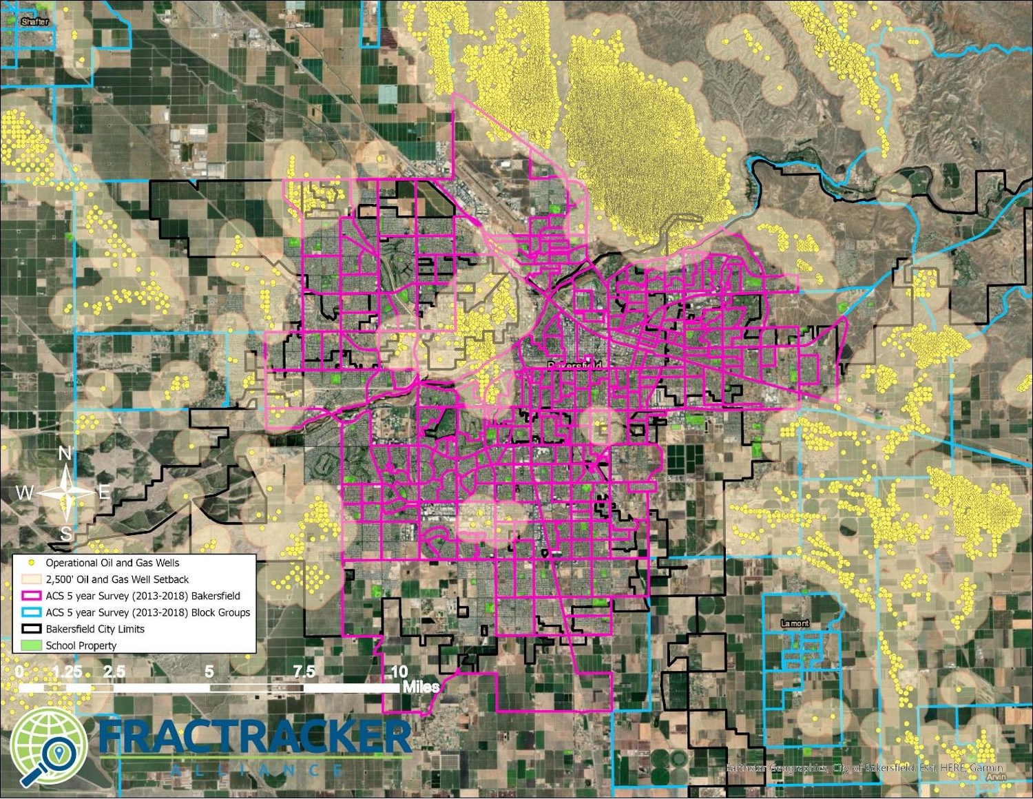
The City of Bakersfield is a unique scenario. It is the largest city in Kern County and as a result suburban developments surround parts of the city. Urban flight has moved much of the wealth into these suburbs. The suburban sprawl has occurred in directions including North toward the Kern River oil field, predominantly on the field’s western flank in Oildale and Seguro. In the map below in Figure 4, these areas are located just to the north of the Kern River.
This is a poignant example of the development of cheap land for housing developments in an area where oil and gas operations already existed; an issue that needs to be considered in the development of setbacks and public health interventions and policies. This small population of predominantly white, middle class neighborhoods shares similar risks as the lower-income Communities of Color who account for the majority of Bakersfield’s urban center. Even though these suburban communities are less vulnerable to the oppressive forces of systemic racism, real estate markets will continue to prioritize cheap land for development, moving communities closer to extraction operations.
Regardless of the implications of urban sprawl and suburban development, it is important to no disregard the risks to the demographics of the at-risk areas of the city of Bakersfield are predominantly Non-white (31%) and Latinx (60%), particularly as compared to the city’s suburbs (15% Non-white and 26% Latinx). About 33,000 people live in the city’s northern suburbs, and another 470,000 live in Bakersfield’s urban city center just to the south of the 16,500 operational wells in the Kern River, Front, and Bluff oil fields. The urban population of Bakersfield is a large Frontline Community exposed to the local and regional negative air quality impacts of the Kern River and numerous other surrounding oil fields.
Figure 4. Map of the city of Bakersfield in Kern County, California located between several major oil fields including the Kern Front oil field. The map shows the 2,500’ setback distance in tan, as well as the census block groups in both pink and blue. Pink block groups show the urban case populations used to generate the demographic summaries.
Southern California
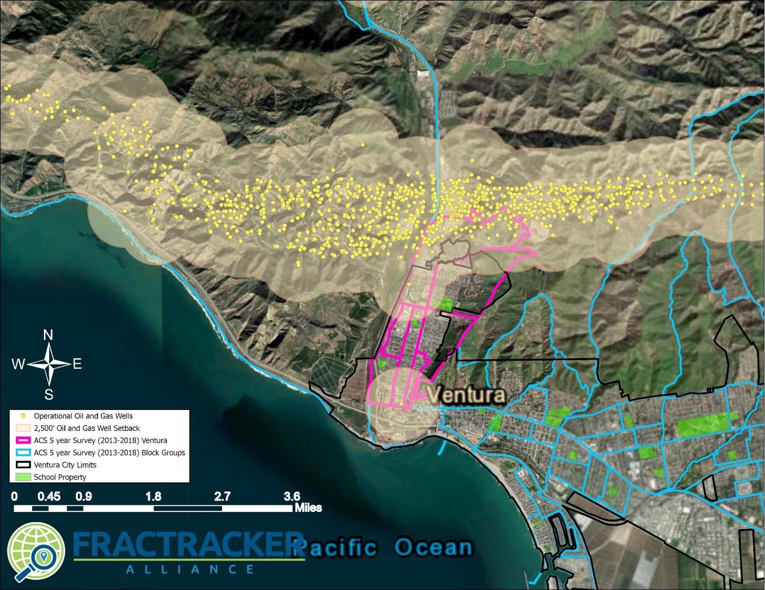
Ventura
The City of Ventura and the proximity of the Ventura oil field is a similar situation to cities in Kern. The urban center of Ventura is bisected by the Ventura oil field’s nearly 1,200 operational wells. While over 70% of the city’s population is Latinx, the very sparsely populated census areas also containing portions of the oil field are 34% Latinx.
In the map below in Figure 5, take note of the population distribution within the portion of the city closest to the oil field versus the census areas to the east. While a statewide or less granular analysis would assume an evenly distributed population density, in this localized analysis, it is clear that the most vulnerable Frontline Communities are the urban centers closest to the oil fields. Even though the census blocks to the east contain oil and gas wells, the populations are less at risk because the population centers are located farther from the oil field.
Figure 5. Ventura Oil Field in Ventura, California census areas within the 2,500’ setback area. The map shows the 2,500’ setback distance in tan, as well as the census block groups in both pink and blue. Pink block groups show the urban case populations used to generate the demographic summaries.
Los Angeles
In Los Angeles County, Inglewood, Wilmington, Long Beach, and Los Angeles City are some of the largest oil and gas fields. There are many areas in Los Angeles where a single low-producing well is located in an upper middle class suburb, on a golf course, or next to the Beverly Hills High School.
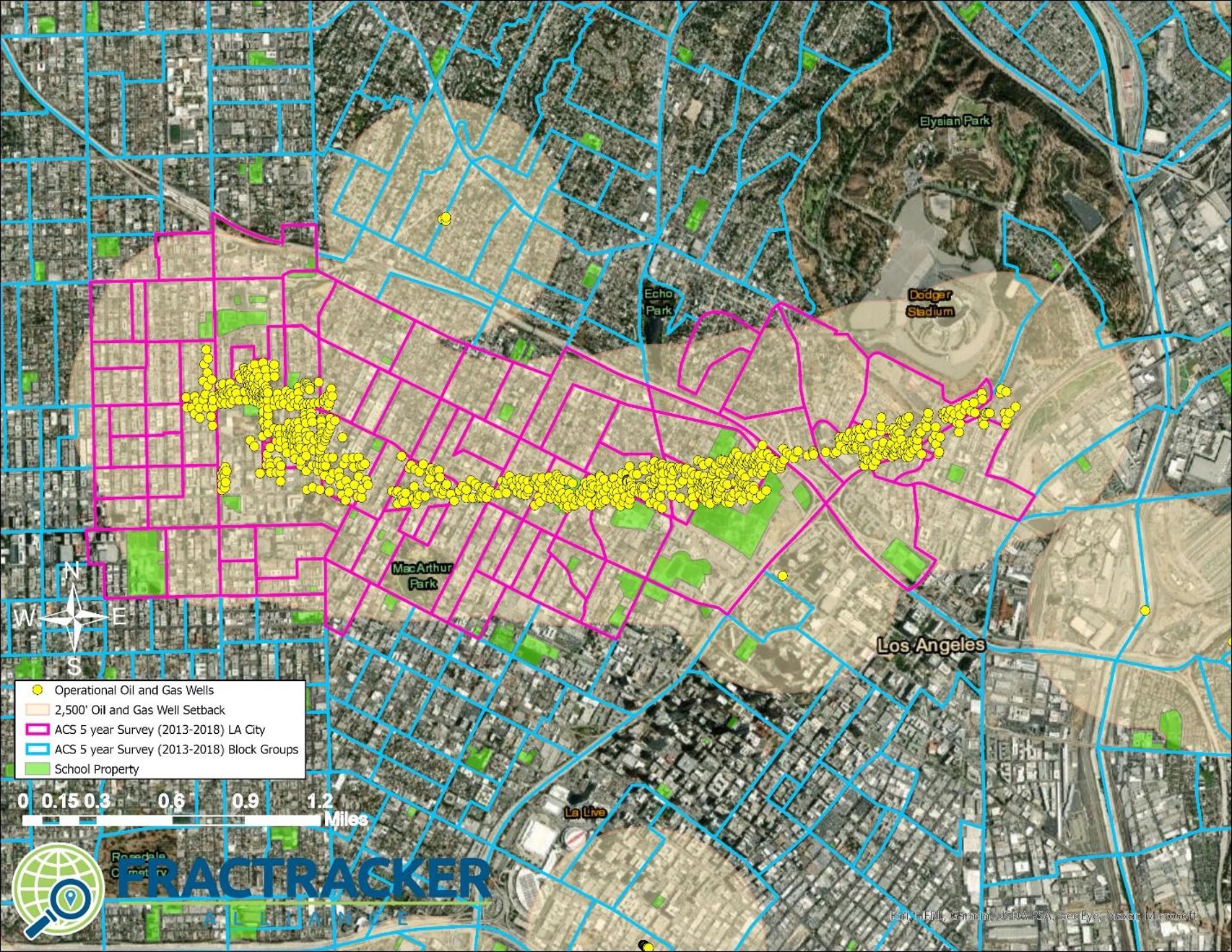
While all well sites present sources of exposure to volatile organic compounds (VOCs) and other air toxics, these four oil fields have incredibly high densities of oil and gas wells in urban neighborhoods. The demographics of the Frontline Communities located within 2,500’ of these major fields are presented below in Table 4. These areas are additionally lower income communities; for example, over 50% of annual household incomes in the census areas surrounding the Los Angeles City oil field are below $40,000, while the Los Angeles County median annual income is over $62,000.
Table 4. Demographics for Frontline Communities living within 2,500’ of Los Angeles’s major oil and gas fields along with counts of operational wells in the fields are shown in the table. The demographic “Latinx” is the count of “Hispanic or Latino Origin” population, and “non-white” was calculated by subtracting “white only” from “total population.”
Oil Field
Well Count
Non-white (%)
Latinx (%)
Inglewood
914
62%
11%
Wilmington
2,995
56%
63%
Long Beach
687
50%
30%
Los Angeles City
872
69%
59%
Ventura
1,193
10%
72%
Toggle between the sections below by clicking in the upper left corner of the title bar.
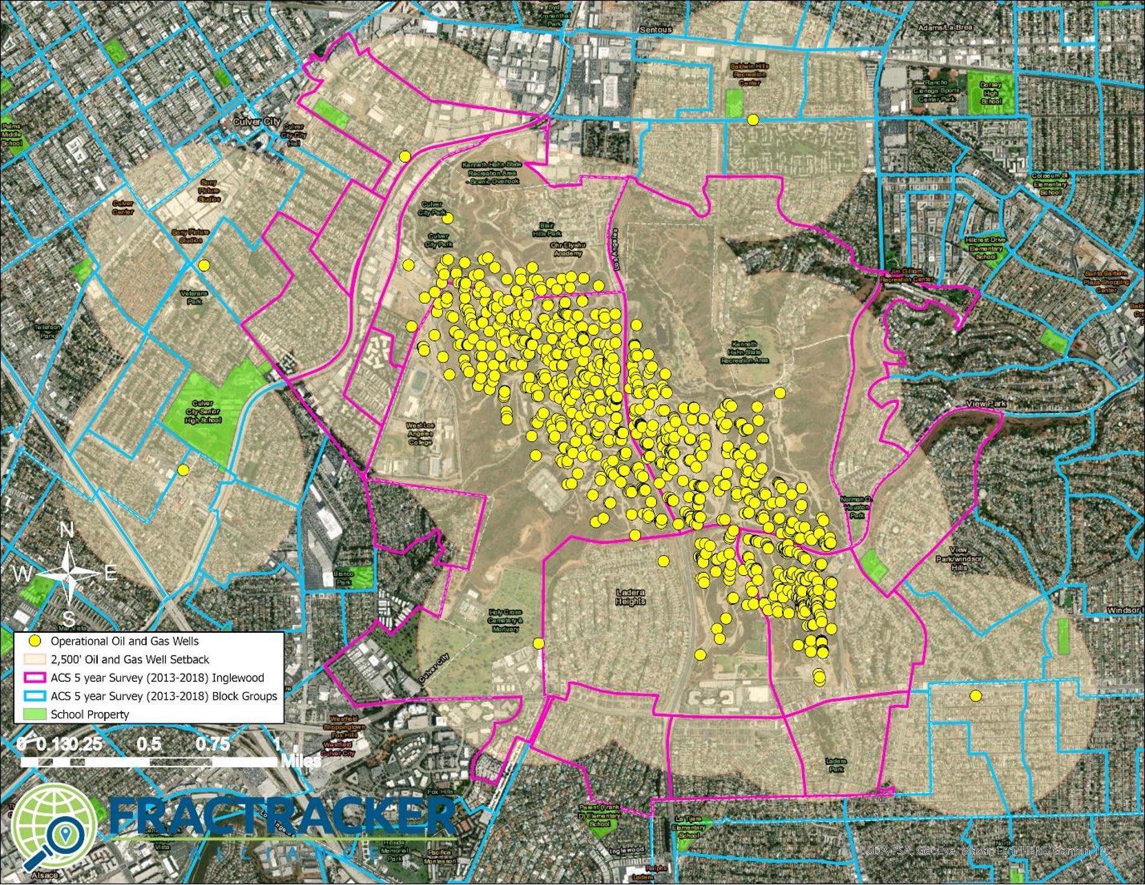
Inglewood
Figure 6. Inglewood Oil Field Frontline Community, Inglewood, California census areas within a 2,500’ setback area. The map shows the 2,500’ setback distance in tan, as well as the census block groups in both pink and blue. Pink block groups show the urban case populations used to generate the demographic summaries.
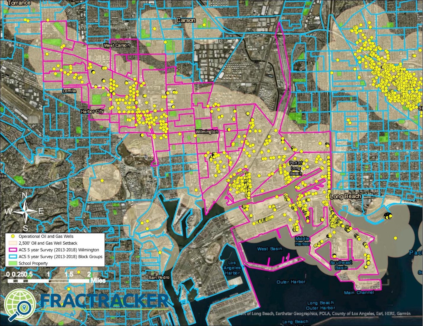
Wilmington
Figure 7. Wilmington Oil Field Frontline Community, Wilmington, California census areas within a 2,500’ setback area. The map shows the 2,500’ setback distance in tan, as well as the census block groups in both pink and blue. Pink block groups show the urban case populations used to generate the demographic summaries.
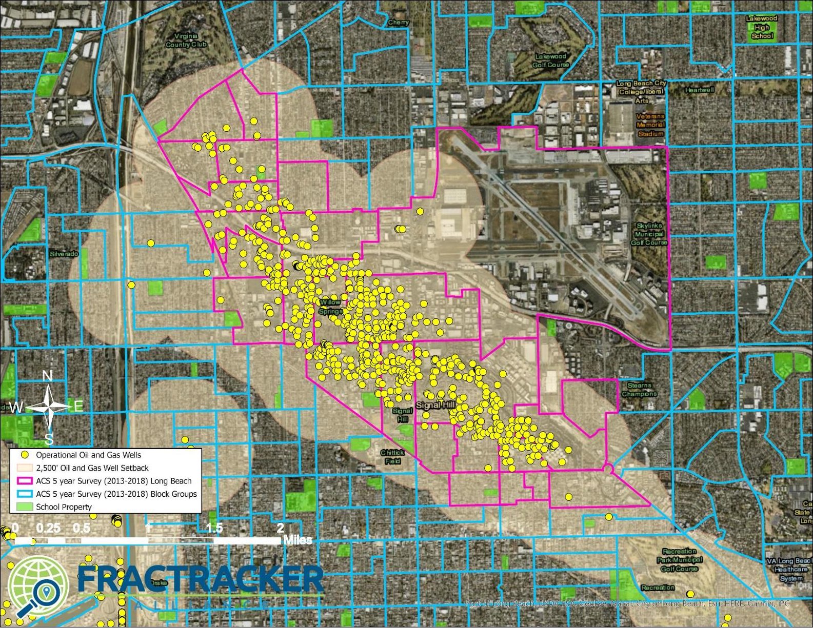
Long Beach
Figure 8. Long Beach Oil Field Frontline Community, Long Beach, California census areas within a 2,500’ setback area. The map shows the 2,500’ setback distance in tan, as well as the census block groups in both pink and blue. Pink block groups show the urban case populations used to generate the demographic summaries.
Los Angeles City
Figure 9. Los Angeles City Oil Field Frontline Community census areas within a 2,500’ setback area. The map shows the 2,500’ setback distance in tan, as well as the census block groups in both pink and blue. Pink block groups show the urban case populations used to generate the demographic summaries.
Production
The creation of public health policies such as 2,500’ setbacks to help protect Frontline Communities is controversial in California as many state legislators are still beholden to the oil and gas industry. The industry itself pushes back strongly against any proposal that could affect their bottom line, no matter how insignificant the financial impact may be. When AB345 was proposed, the industry’s lobbying organization Western States Petroleum Association claimed that institution of 2500’ setbacks would immediately shut down at least 30% of California’s total oil production. This number is an outright fabrication.
As shown in Table 1 above, a 2,500’ setback would impact the less than 9,000 active and new wells; 42% in Kern County and 29% in Los Angeles County. Ventura and Orange Counties are a distant 3rd and 4th, respectively. These counts are further broken down by field in Table 5 below. Statewide these wells accounted for just 12.8% of California’s current oil production by volume (as reported in barrels of oil/condensate by CalGEM), which is much smaller than the wholly unsubstantiated 30% decline claimed by industry.
Table 5. Counts of wells by well status for operational (active, idle, and new) oil and gas wells located within a 2,500’ setback. Fields include the count of wells within the 2,500’ setback and the amount of oil produced from those wells within the setback. The percentage of total oil from that field is also included.
Oil Field
County
Well Count
Well Ct % of Total
2019 Oil Prod (BBLS)
Oil Prod % of Total
Wilmington
Los Angeles
2,514
83%
2,292,669
22%
Kern River
Kern
1,338
9%
2,121,071
12%
Inglewood
Los Angeles
891
97%
1,806,354
96%
Midway-Sunset
Kern
1,892
10%
1,614,081
8%
Ventura
Ventura
287
24%
1,202,764
31%
Long Beach
Los Angeles
687
100%
1,036,506
100%
Brea-Olinda
Los Angeles
695
97%
967,223
95%
Huntington Beach
Orange
528
83%
753,494
42%
Placerita
Los Angeles
448
100%
508,182
100%
Santa Fe Springs
Los Angeles
304
99%
421,719
72%
Cat Canyon
Santa Barbara
115
10%
418,697
36%
Beverly Hills
Los Angeles
156
100%
351,877
100%
McKittrick
Kern
334
18%
346,738
10%
Montebello
Los Angeles
227
98%
318,657
97%
Fruitvale
Kern
286
80%
316,184
75%
San Ardo
Monterey
180
13%
313,339
4%
Torrance
Los Angeles
219
100%
307,413
100%
Seal Beach
Los Angeles
175
88%
282,790
74%
Shafter, North
Kern
70
78%
267,256
66%
Edison
Kern
520
41%
261,098
39%
Brentwood
Contra Costa
4
100%
230,868
100%
Oxnard
Ventura
124
82%
214,884
100%
Sansinena
Los Angeles
162
100%
207,474
100%
Poso Creek
Kern
320
16%
193,533
4%
Rosecrans
Los Angeles
94
100%
174,720
100%
Rio Bravo
Kern
80
74%
166,444
82%
Richfield
Orange
231
100%
165,426
100%
Coyote, East
Orange
81
100%
163,639
100%
San Vicente
Los Angeles
48
100%
162,940
100%
In the case that setback regulations are crafted both to prohibit new drilling and to phase out existing operations within the setback distance, the industry would have the opportunity to respond with measures that preserve the majority of production volumes, particularly in the Central Valley. For example, in Kern County, the overwhelming majority of new wells drilled in 2020 are directional or horizontal; these drilling technologies would allow operators to access the same below ground resources from surface locations that are further away from and safer for communities. Further, for existing wells within the 2,500’ setback, current proposals would institute a phase out period. Existing wells could be allowed to continue to operate under the terms of their current permits but not allowed to expand or rework their operations to increase or extend production; alternatively (or in addition), well operators could continue for a prescribed timeframe formulated to allow them to recoup their investment (called “amortization”).
Los Angeles
It is clear that the oil fields of Los Angeles would be the most impacted if setbacks phased out the wells responsible for the highest risk to Frontline Communities. The majority of Los Angeles’s urban oil fields are located entirely within 2,500’ of homes, schools, healthcare facilities and daycares.
As shown above in Table 5, wells within the setback produce 96% of the oil in the Inglewood fields, 84% in the Long Beach field, and 100% of the oil in several other smaller fields. With the phase out of these wells, oil extraction would cease in these fields. Most of these fields produce very low volumes of oil and already have high counts of idle wells, 28% idle in Wilmington, 25% in Inglewood, and 56% in Long Beach for example. The sole outlier of this trend is the Wilmington field. The majority of production in the Wilmington field comes from wells located in the Long Beach harbor, enough of them located outside of the 2,500’ setback such that while 83% of the Wilmington field wells are within the 2,500’ setback, these wells account for only 22% of the field’s overall production.
Kern County
The situation in Kern County is quite the opposite of Los Angeles, where the majority of operational wells are located within 2,500’ of homes, residences, and other sensitive receptors like healthcare facilities. In Kern, the overwhelming majority of wells are located beyond 2,500’ and even 1 mile from sensitive receptors. While the Midway-Sunset and Kern River fields have the most wells within the 2,500’ setback area, those wells make up a small percentage of the total operational wells in the fields. As can be seen in the map in Figure 1, wells within the 2,500’ setback zone in the large Kern oil fields are entirely located on the borders of the fields. Overall, a 2,500’ setback in Kern County would only affect 7.1% of active/new wells, accounting for 5.97% of the county’s production.
The oil and gas industry and operators in states including Texas, Colorado, North Dakota, Pennsylvania, Ohio, West Virginia, New Mexico, and Oklahoma are very vocal of their ability to avoid surface disturbance and target oil and gas pools located under sensitive receptors (homes, schools, healthcare facilities, endangered species habitat etc.) using directional drilling. According to the industry, directional drilling has been used for nearly a century to extract resources from areas where surface disruption would impact sensitive communities and habitats.
The same is true for California, especially in Kern County and especially recently. An October 2020 draft environmental impact report by the Kern County Planning and Natural Resource Department disclosed that in a dataset of 9,803 wells drilled from 2000 to 2020 by the California Resources Corporation, the majority of wells were drilled directionally (46%) or horizontally (10%), as opposed to vertically. More recent wells in the County have utilized directional and horizontal drilling even more heavily: a 2020 dataset of wells drilled county-wide indicates that 76% were drilled directionally and an additional 7% were drilled horizontally; only 17% were drilled vertically. These statistics indicate that, even if all wells neighboring Frontline Communities in Kern County were to be phased out (itself a small percentage of the total number of wells in the county), there would only be a small impact on Kern County oil production owing to the prevalence of non-vertical techniques that allow operators the flexibility to access reserves from different surface locations. As noted previously, if all oil production from within the 2,500’ setback zone were to be immediately eliminated statewide, it would mean a maximum decrease of just 12.8% of California’s current annual oil production. But the availability of directional and horizontal drilling in Kern County, where the lion’s share of all drilling statewide occurs, means it is more likely that the decrease in production will be significantly less than 12.8% and likely much less than 10%.
Existing Well Phase Out
Any assertion that a 2,500’ setback would immediately affect oil production is baseless because current setback proposals would institute a phase out period for existing wells. For example, existing permitted wells could be allowed to continue to operate under the terms of their current permits but not allowed to expand or rework their operations to increase or extend production. Alternatively, under a policy approach known as amortization, well operators could continue for a prescribed timeframe formulated to allow them to recoup their investment.
If wells within the setback distance are phased out pursuant to a “no rework” policy, operators would be afforded some time to maximize production in order to ensure that operators receive a sufficient return on their investment under the terms of their existing permits before they shut down. Under such an approach, older wells with increasing risks of fugitive emissions through leaks at the surface and well casing failures could be sequentially phased out by placing a ban on rework permits not required for maintenance or safety. CalGEM permitted well reworks, including sidetracks and deeper drills, increase production and the lifespan of wells. The catalog of rework permits can be found on the CalGEM website.
Based on CalGEM’s production data from 2018 and 2019, a phase out effectuated by disallowing well reworks would result in an annual reduction of less than 1% of total oil production. Of the 52,997 wells reporting oil/condensate production volumes in 2018, 338 received a rework permit in the same year. In 2019, of the 48,860 wells reporting oil production volumes, 285 received rework permits. By volume, the wells that received rework permits accounted for 0.87% of oil production in 2018 and just 0.04% in 2019.
Conclusion
The oil and gas industry in California has consistently pushed back against Frontline Communities who demand public health protections against emissions from oil and gas operations. This occurs even when there will be little to no impact reducing production. It is an industry policy to refuse any concessions and oppose all measures, even to protect public health, by leveraging the industry’s wealth at every level of the political hierarchy.
Fatefully, 2020 has resulted in multiple wins for public health in California. While the failure of AB345 made it clear that the California state legislature is still beholden to the fossil fuel industry, the momentum has continued. Community grassroots groups in Ventura County successfully passed a 1,500’ setback ordinance for occupied dwellings and 2,500’ setbacks for sensitive receptor sites including healthcare facilities and schools. Just south of Ventura, the County of Los Angeles is also in the midst of a rule-making process that is considering multiple setbacks, including 1,000’ to 2,500’ distances. And a committee of the Los Angeles City Council just voted to develop a proposal that would phase out oil drilling across the city as a non-conforming use.
While Ventura and Los Angeles are making progress, Kern County is creating a new process to streamline oil and gas well permitting and has even proposed to decrease the existing zone-specific 300’ setbacks from homes to 210’.
Kern County Frontline Communities and the rest of California also deserve the same consideration as residents of Ventura and Los Angeles Counties. The research is clear that a setback of at least one mile in addition to more site specific public health interventions are necessary to reduce the negative health impacts resulting from these industrial operations within and neighboring Frontline Communities.
https://www.fractracker.org/a5ej20sjfwe/wp-content/uploads/2020/12/CASetbacksMappic.jpg6141500Kyle Ferrar, MPHhttps://www.fractracker.org/a5ej20sjfwe/wp-content/uploads/2025/09/2025-Wordmark-Logo.pngKyle Ferrar, MPH2020-12-17 13:45:242021-04-15 14:16:02People and Production: Reducing Risk in California Extraction
Working with the environmental nonprofit Earthworks, FracTracker Alliance filmed emissions from oil and gas sites that have been issued permits in California under Governor Gavin Newsom since the beginning of 2019. Using state-of-the-art technology called optical gas imaging (OGI), we documented otherwise invisible toxic pollutants and greenhouse gas emissions (GHGs) being released from oil and gas wells and other infrastructure. This powerful technology provides further evidence of the negative consequences that come from each issued permit. Every single permit approval enabled by decisions made under Newsom can have substantial, visible impacts on local and regional air quality, contributes to climate change, and potentially exposes communities to health-harming pollution.
Despite a stated commitment to transition rapidly off fossil fuels, California has issued 7,625 permits to drill new oil and gas wells and rework existing wells since the beginning of 2019 — that is, on Governor Gavin Newsom’s watch. This expansion of the industry has clear implications for climate change and public health, as this article will demonstrate.
Intro
In collaboration with Consumer Watchdog, FracTracker Alliance has been periodically reporting on the number and locations of oil and gas wells permitted by Governor Newsom in California. In July of 2019, we showed how the rate of fracking under Governor Newsom had doubled, as compared to counts under former Governor Brown. Since then we have continued tracking the numbers and updating the California public via multiple news stories, blog reports, and with a map of new permits on NewsomWellWatch.com, where permitting data for the third quarter of 2020 has just been posted.
Now again, the rate of new oil and gas well permits issued by the California Geologic Energy Management division (CALGEM) continues to increase even faster in 2020, with permits issued to drill new oil and gas production wells nearly doubling since 2019. But what exactly does this mean for Frontline Communities and climate change? To answer this question, FracTracker Alliance and Consumer Watchdog teamed up with Earthworks’ Community Empowerment Project (CEP).
CEP’s California team worked with community members and grassroots groups to film emissions of methane and other volatile organic compounds (VOCs) emitted from oil and gas extraction sites, including infrastructure servicing oil and gas production wells such as the well-heads, separators, compressors, crude oil and produced water tanks, and gathering lines. Emissions of GHGs, such as methane, are a violation of the California Air Resources Board’s (CARB) California oil and gas rule (COGR), California Code of Regulations, Title 17, Division 3, Chapter 1, Subchapter 10 Climate Change, Article 4, § 95669, Leak Detection and Repair.
The emissions were filmed by a certified thermographer with a FLIR (Forward Looking Infrared) GF320 camera that uses optical gas imaging (OGI) technology. The OGI technology allows the camera to film and record visualizations of VOC emissions based on the absorption of infrared light. It is the exact same technology required by the U.S. EPA under the rule for new source performance standards and the by California Air Resources Board for Leak Detection and Repair (LDAR) to properly inspect oil and gas infrastructure. The video footage clearly shows the presence of a range of VOCs, methane, and other gases that are otherwise invisible to the naked eye.
The footage shown below is in greyscale and can appear grainy when the camera is being operated in high sensitivity modes, which is sometimes necessary to visualize certain pollution releases. The descriptions preceding each video explain what the trained camera operator saw and documented. A map of these sites is presented at NewsomWellWatch.com.
Newsom Well Watch interactive map
Navigate to the next slide using the arrows at the bottom of the map.
Find the story map, and more by clicking the image below.
Case Studies on Permitted Sites
Cat Canyon Tunnell Well Pad.
Earthworks’ California CEP thermographer visited this site in December of 2019, and just happened to arrive while the operator (oil and gas company) was conducting activities underground, including drilling new wells and reworking existing wells. In 2019 the operator, Vaquero Energy, was approved to drill 10 new cyclic steam wells and rework 23 existing oil and gas production wells at this site.
The footage shows significant emissions coming from an unknown source near the wellheads on the well pad; most likely these emissions were coming directly from the open boreholes of the wells. The emissions potentially include a cocktail of VOCs and GHGs such as methane, ethane, benzene, and toluene. This footage provides a candid view of what is released during these types of activities. The pollution shown appears to be the result of an uncontrolled source commonly resulting from drilling and reworking wells
Additionally, inspectors are rarely, if ever, present during these types of activities to ensure that they are conducted in accordance with regulations. The CEP camera operator reported the emissions and provided the OGI video to the Santa Barbara County Air Pollution Control District. By the time the inspector arrived, however, the drilling crew had ceased operations. The inspector did not detect any of these emissions, and as a result the operator was not held accountable for this large pollution release.
In the footage below, the emissions can be seen traveling over the fenceline of the well pad, swirling and mixing with the wind. This site is a clear example of what to look for in the following videos, since the emissions are so obvious. Fortunately, there are no homes or buildings in close proximity to this site, which potentially limited direct pollution exposure — although the pollution still degrades air quality and can pose an occupational health risk to oil field workers.
South Los Angeles Murphy Drill Site
The Murphy Drill Site in Los Angeles has been a long-standing nuisance and source of harmful pollution for neighbors in Jefferson Park. The site houses 31 individual operational wells, including 9 enhanced oil recovery injection wells and 22 oil and gas production wells, as shown below in the map in Figure 1. The wells are operated by Freeport-McMoran, while the site is owned by the Catholic archdiocese of Los Angeles. The site is within 200 feet of homes, playgrounds and a health clinic. There are over 16,000 residents within 2,500’ of the site, as well as a special needs high school, an elementary school, a hospice facility, and a senior housing complex.
Figure 1. Map of the Murphy drill site
The neighborhoods near the Murphy Site are plagued with strong chemical odors, including those linked to oil and gas operations (such as the “rotten egg” smell of health-harming hydrogen sulfide), most likely from the toxic waste incinerators on site. Community members have suffered from respiratory problems, chronic nosebleeds, skin and eye irritation, and headaches. The operators have received multiple violations, including for releasing emissions at concentrations 400% over the allowable limit of methane and VOCs. Some of these violations were the direct result of complaints from the community and the Earthworks CEP team, which filmed pollution from the site on multiple occasions. Yet despite receiving “Notices of Violations” and fines, Freeport-McMoran has been allowed to continue operations. In OGI footage, emissions are visible continuously escaping from a vent on the equipment. While this leak has been addressed by regulators, each new visit to this site tends to result in finding new uncontrolled emissions sources.
South Los Angeles Jefferson Drill Site
The Jefferson drill site is very similar situation to the Murphy Site. The sites have the same operator, Freeport-McMoran, and surrounding neighborhoods in both locations have suffered from exposure to toxic pollution as well as odors, truck traffic, and noise. The Jefferson site has 49 operational wells, including 15 enhanced oil recovery wells, as shown below in Figure 2. In 2013 the operator reported using over 130,000 pounds of corrosive acids and other toxic chemicals for enhanced oil recovery operations. Regardless, an environmental impact report has never been completed for this site.
Figure 2. Map of the Jefferson drill site in South Los Angeles.
The site is located 3 feet from the nearest home, and the surrounding residential buildings are considered “buffers” for the rest of the neighborhood, which also includes an elementary school about 700 feet away. The site was nearly shut down by the City of Los Angeles in 2019, but is currently still operational. In 2019 the site was even issued a permit to rework an existing well in order to increase production from the site. The footage below shows a large, consistent release of pollution from equipment on the well pad. The plume appears above the site and is visible against the background of the sky. The Earthworks CEP team reported the pollution to the South Coast Air Quality Management District (SCAQMD), which conducted an inspection, stopped the leak, and issued a notice of violation and a fine. It is not clear exactly how long this pollution problem had gone unnoticed or unaddressed, and it is not unlikely that another leak will occur without being quickly identified.
Wilmington E&B Resources WNF-I Site on Main St
The WNF-I drilling site is located in Carson in the City of Los Angeles. Operated by E&B Natural resources in the Wilmington oil and gas field, the site houses 35 operational oil and gas wells, including 12 enhanced oil recovery wells and a wastewater disposal well. There is also extensive above-ground infrastructure on the well site, including a large, high-volume tank battery used to store oil and wastewater produced from numerous oil and gas wells in the area.
Using OGI, Earthworks identified a large pollution release from the top of the largest tank. In the video footage, the plume or cloud of gases (likely methane and VOCs) can be seen hovering over the site and slowly dispersing over the fence-line into the communities of West Carson and Avalon Village. Despite clear operational problems, CalGEM approved this site for two rework permits in 2019 and then three re-drills (known as sidetracks) of existing wells in 2020 in order to increase production. The SCAQMD reports that they have inspected this facility, but it is not clear whether this major uncontrolled source has been stopped.
Long Beach Signal Hill Drill Site
At an urban drilling site in the neighborhood of Signal Hill in Los Angeles County, Earthworks filmed and documented pollution releases from numerous pieces of equipment. The site includes 15 operational oil and gas wells operated by Signal Hill Petroleum and The Termo Company. Emissions of gases (likely methane and VOCs) were documented on infrastructure from both operators. At this site, Signal Hill Petroleum received a permit in April 2019 to rework an operational well to increase production. That well is located less than 70’ from a home.
While this site is located within Los Angeles County, it is outside the jurisdiction of the city itself. Any local protections for drilling sites within the Los Angeles city limits are not afforded to communities such as Signal Hill. This area that includes the Signal Hill oil field and the Signal Hill portion of the Long Beach oil field, where many well sites are unmaintained and oversight is limited — conditions that in turn can result in corrosion and pollution leaks. The SCAQMD inspected this site and reported that these uncontrolled sources of emissions have been addressed by the operator, but it is not clear if the emission have stopped.
Midway-Sunset Crail Tank Farm
This tank farm, located in Kern County, services a number of wells operated by Holmes Western Oil Corporation on the outskirts of the Mid-Way Sunset Field. Of the wells serviced by this site, permits were issued to four active oil and gas production wells in 2019. The permits authorized the operator to rework the wellbores in order to increase production. The site contains nine operational oil and gas wells, including eight production wells pumping oil to the surface and one wastewater disposal well. There are multiple homes near this site, within 400’ to the west and within 300’ to the northeast.
For each gallon of oil produced, another ten gallons of contaminated wastewater are brought to the surface. Using diesel or gas generators this wastewater is pumped back into the ground. California regulators have a bad track record of managing underground injection of wastewater, which is now under the U.S. EPA’s oversight. The groundwater in this area of Kern County is largely contaminated and considered a sacrifice zone.
The emissions from this site are from the pressure release valves on the tops of multiple tanks. The tanks store both crude oil and wastewater. The infrared spectrum allows the camera to film the tank levels, which are nearly full. As the tanks fill with more crude oil and hydrocarbon contaminated wastewater the head space of the tank pressurizes with more VOC’s. This footage was also filmed at night when emissions are typically much lower. During the day heat from the sun (radiative energy) heats the tanks and increases the head space pressure resulting in greater emissions. While the San Joaquin Valley Air Pollution Control District (SJVAPCD) was notified of these uncontrolled sources of emissions, their own inspections of the site did not identify an actionable offense on the part of the operator and these uncontrolled emissions continue to be released.
Tank Emissions
Crude oil and wastewater storage tanks are a common source of fugitive emissions and represent the majority of emissions presented in this report. Some tanks and well-sites use best practices that include closed vapor recovery systems to prevent venting tanks from leaking, but the vast majority do not and vent directly to the atmosphere. In all cases, tanks and pipeline infrastructure use pressure release valves to vent emissions when pressure builds too high. This venting is permitted as strictly an emergency activity to prevent hazardous build-up of pressure. Vents are even designed to open and reset themselves automatically. Consequently, tank venting is a common practice and operators seem to often leave these valves open.
While the recently enacted California Oil and Gas Rule (COGR) places limits on GHG emissions from all oil and gas facilities, internal policy of the San Joaquin Air Valley Air Pollution Control District has previously exempted tanks at low-producing well sites from having to be kept in a leak-free condition, creating a regulatory conflict that air districts and CARB need to resolve. This type of emissions source is also difficult for regulators to identify during inspections, for a number of reasons. These valves are typically located on the tops of large tanks where they are difficult to access and view, and inspections and sampling can only occur by chance (i.e., when the valve in open). Further, these valves can be immediately closed by operators during or upon notification of an upcoming inspection.
New Permits: Moving in the Wrong Direction
When Earthworks CEP uses OGI cameras to inspect an oil and gas site in California, finding and documenting pollution releases is so common that it is the default expectation. Because of access and proximity limitations, it is possible that more pollution is being released from sites than CEP can identify. All of these examples of pollution, including releases of methane and VOCs, add up to potentially degrade air quality and expose Frontline Communities to health risks — as well as many others just like them. This summary represents a small collection of leaking well sites visited by Earthworks CEP, which have coincidentally received new permits to operate and rework existing wells since January 1, 2019. CEP has also documented many other hazardous cases, such as the Jewett 1-23 site in Arvin (shown in the footage below), that is persistently exposing elementary school students to VOCs. These sites surely make up only a small proportion of the polluting oil and gas sites in California that harm climate and health.
From the initial drilling of an oil and gas well, during production, and into subsequent reworks, all phases of a well’s lifetime result in unpermitted and undocumented fugitive emissions. Regulating emissions from oil and gas extraction operations has not been effective in California. Regardless of notices of violations and fines, polluting facilities and well sites continue to operate and even receive new permits. Even the COGR rule, lauded as the most stringent GHG emissions regulation in the nation is technically unable to eliminate or even identify these uncontrolled sources. It is clear that the only ways to reduce exposures to these emissions for Frontline Communities is to institute protective setbacks and stop permitting the drilling of new wells and the reworking of aging wells.
https://www.fractracker.org/a5ej20sjfwe/wp-content/uploads/2019/08/EQT-Tioga-Wide-7.gif300800Kyle Ferrar, MPHhttps://www.fractracker.org/a5ej20sjfwe/wp-content/uploads/2025/09/2025-Wordmark-Logo.pngKyle Ferrar, MPH2020-11-18 12:40:132021-04-15 14:16:04Documenting emissions from new oil and gas wells in California
FracTracker’s Ted Auch coauthored a recent article in the journal Democracy & Security that considers the US shale oil and gas industry through a national security lens.
This paper was authored by Bryan T. Stinchfield , Ted Auch & Eve Bratman.
Proponents of the US shale oil and gas industry argued that American citizens’ economic prosperity and national security were at stake if the industry was not rapidly expanded. Following copious amounts of a certain type of “patriotic” rhetoric, the industry grew rapidly. Simultaneously, foreign ownership of US shale industry infrastructure occurred in tandem with calls for new policies and laws to limit US citizens’ democratic rights with regard to the industry’s activities. As a result, we argue that the development of the US shale industry has weakened national security by creating negative security externalities and eroding democratic values. We offer implications for other democratic societies rich in natural resources.
Figure 1. Vicious cycle within the US shale industry.
The intent of some of the industry’s proponents is to criminalize protest, peaceful and otherwise. When peaceful protests are intentionally lumped in with not-peaceful protests, the effect is a weakening of democracy.
Energy Security, International Investment, and Democracy: The Case of the United States Shale Oil and Gas Industry
Bryan T. Stinchfield , Ted Auch & Eve Bratman
To cite this article: Bryan T. Stinchfield , Ted Auch & Eve Bratman (2020): Energy Security, International Investment, and Democracy: The Case of the United States Shale Oil and Gas Industry, Democracy and Security, DOI: 10.1080/17419166.2020.1811969
To link to this article: https://doi.org/10.1080/17419166.2020.1811969
https://www.fractracker.org/a5ej20sjfwe/wp-content/uploads/2020/10/TAuch_infrastructure-wellpad-sandtruck-ChesapeakeAppalachia-RainSulWellpad-SullivanCounty-PA_July2020-feature-scaled.jpg6671500Ted Auch, PhDhttps://www.fractracker.org/a5ej20sjfwe/wp-content/uploads/2025/09/2025-Wordmark-Logo.pngTed Auch, PhD2020-10-15 11:24:272021-04-15 14:16:07Energy Security, International Investment, and Democracy in the US Shale Oil & Gas Industry
In this special one-day fundraiser event, two intrepid FracTracker teams will build and share a live virtual map as we travel throughout the Ohio River Valley Region documenting oil, gas, and its effects on our health, climate, and environment.
How many sites can we visit in one day? What will we find?
We’ll share our findings to build awareness about the plight of this region—and so many other places victimized by this rogue industry. Plus, viewers will gain a firsthand understanding of how FracTracker turns data into real-world impact.
Proceeds will benefit the ongoing work of FracTracker to decarbonize our economy and promote environmental justice.
Whether you are able to contribute financially at this time or not, we hope you’ll join us on this virtual journey. You’ll see regular video updates along the way as we share our progress, and watch as a story map is updated throughout the day.
Join our team of explorers in spirit and pledge your support! We’re excited to share this journey with you.
https://www.fractracker.org/a5ej20sjfwe/wp-content/uploads/2020/08/FracTracker-in-the-Field-promotion5-scaled.jpg8441500FracTracker Alliancehttps://www.fractracker.org/a5ej20sjfwe/wp-content/uploads/2025/09/2025-Wordmark-Logo.pngFracTracker Alliance2020-08-14 12:44:552021-04-15 14:16:11FracTracker in the Field: Building a Live Virtual Map
As a spring 2020 intern with FracTracker, my work mostly involved mapping gathering lines in West Virginia and Ohio. Gathering lines are pipelines that transport oil and gas from the wellhead to either compressor stations or storage/processing facilities. The transmission pipelines (which are often larger in diameter than gathering lines) take the oil and gas from the processing facilities to other storage facilities/compressor stations, or to distribution pipelines which go to end users and consumers. As you can see from Figure 2 in the map of Doddridge County, WV, many gathering lines eventually converge at a compressor station. You can think of gathering lines like small brooks and streams that feed transmission pipelines. The transmission lines are the main arteries, like a river, moving larger quantities of gas and oil over longer distances.
PROJECT DESCRIPTION
The main project and goal of my internship was to record as many gathering pipelines as I could find in Ohio and West Virginia, since gathering lines are not generally mapped and therefore not easily available for the public to view. For example, the National Pipeline Mapping System’s public map viewer (created by the Department of Transportation Pipeline and Hazardous Materials Safety Administration) has a note stating, “It does not contain gas gathering or distribution pipelines.” Mapping gathering lines makes this data accessible to the public and will allow us to see the bigger picture when it comes to assessing the environmental impact of pipelines.
After collecting gathering line location data, I performed GIS analysis to determine the amount of acreage of land that has been clearcut due to gathering pipeline installations.
Another analysis we could perform using this data is to count the total number of waterways that the gathering lines cross/interact with and assess the quality of water and wildlife in areas with higher concentrations of gathering pipelines.
Figure 1. This map shows an overview of gathering line pipelines in the Powhatan Point, Ohio and Moundsville, West Virginia of the Ohio River Valley.
PIPELINE GATHERING LINE MAPPING PROCESS
I worked with an aerial imagery BaseMap layer (a BaseMap is the bottommost layer when viewing a map), a county boundaries layer, production well location points, and compressor station location points. I then traced lines on the earth that appeared to be gathering lines by creating polygon shapefiles in the GIS application ArcMap.
My methodology and process of finding the actual routes of the gathering lines included examining locations at various map scale ranges to find emerging line patterns of barren land that connect different production well points on the map. I would either concentrate on looking for patterns along well pad location points and look for paths that may connect those points, or I would begin at the nearest gathering line I had recorded to try to find off-shoot paths off of those pipelines that may connect to a well pad, compressor station or previously recorded gathering line.
I did run into a few problems during my search for gathering lines. Sometimes, I would begin to trace a gathering line path, only to either loose the path entirely, or on further inspection, find that it was a power line path. Other times when using the aerial imagery basemap, the gathering line would flow into an aerial photo from a year prior to the pipeline installation and I would again lose the path. To work around these issues, I would first follow the gathering line trail to its end point before I started tracing the path. I would also view the path very closely in various scale ranges to ensure I wasn’t tracing a road, waterway, or powerline pathway.
ACREAGE ANALYSIS
In the three months that I was working on recording gathering pipeline paths in Ohio and West Virginia, I found approximately 29,103 acres (3,494 miles) of barren land clearcut by gathering pipelines. These total amounts are not exact since not all gathering lines can be confirmed. There are still more gathering lines to be recorded in both Ohio and West Virginia, but these figures give the reader an idea of the land disturbance caused by gathering lines, as shown in Figures 1 and 2.
In Ohio, I recorded approximately 10,083 acres (641 miles) with the average individual gathering pipeline taking up about 45 acres of land. With my gathering line data and data previously recorded by FracTracker, I found that there are 28,490 acres (1,690 miles) of land spanning 9 counties in southeastern Ohio that have been cleared and used by gathering lines.
For West Virginia, I was able to record approximately 19,020 acres (1,547 miles) of gathering lines, with the average gathering line taking up about 48 acres of space each. With previous data recorded in West Virginia by FracTracker, the total we have so far for the state is 22,897 acres (1,804 miles), although that is only accounting for the 9 counties in northern West Virginia that are recorded.
Figure 2. This aerial view map shows connecting gathering line pipelines that cover a small portion of Doddridge County, WV.
CONCLUSION
I was shocked to see how many gathering lines there are in these rural areas. Not only are they very prevalent in these less populated communities, but it was surprising to see how concentrated and close together they tend to be. When most people think of pipelines, they think of the big transmission pipeline paths that cross multiple states and are unaware of how much land that the infrastructure of these gathering pipelines also take up.
It was also very eye-opening to find that there are at least 29,000 acres of land in Ohio and West Virginia that were clearcut for the installation of gathering lines. It is even more shocking that these gathering pipelines are not being recorded or mapped and that this data is not publicly available from the National Pipeline Mapping System. While driving through these areas you may only see one or two pipelines briefly from your car, but by viewing the land from a bird’s eye perspective, you get a sense of the scale of this massive network. While the transmission pipeline arteries tend to be bigger, the veins of gathering lines displace a large amount of land as well.
I was also surprised by the sheer number of gathering lines I found that crossed waterways, rivers, and streams. During this project, it wasn’t unusual at all to follow a gathering line path that would cross water multiple times. In the future, I would be interested to look at the number of times these gathering pipelines cross paths with a stream or river, and the impact that this has on water quality and surrounding environment. I hope to continue to record gathering lines in Ohio and West Virginia, as well as Pennsylvania, so that we may learn more about this infrastructure and the impact it may have on the environment.
About Me
I first heard of FracTracker three years ago when I was volunteering with an environmental group called Keep Wayne Wild in Ohio. Since learning about FracTracker, I have been impressed with their eye-opening projects and their ability to make the gas and oil industry more transparent. A few years after first hearing about FracTracker, and as my interest in the GIS field continued to grow, I began taking GIS classes and reached out to them for this internship opportunity.
By Trevor Oatts, FracTracker Spring 2020 Data & GIS Intern
https://www.fractracker.org/a5ej20sjfwe/wp-content/uploads/2020/07/Mapping-gathering-lines-in-OH-and-WV-feature.jpg8331875Intern FracTrackerhttps://www.fractracker.org/a5ej20sjfwe/wp-content/uploads/2025/09/2025-Wordmark-Logo.pngIntern FracTracker2020-07-02 12:09:192025-05-02 14:45:00Mapping Gathering Lines in Ohio and West Virginia
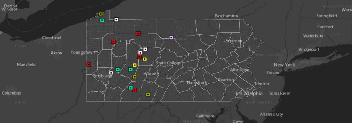 FracTracker Alliance, 2021
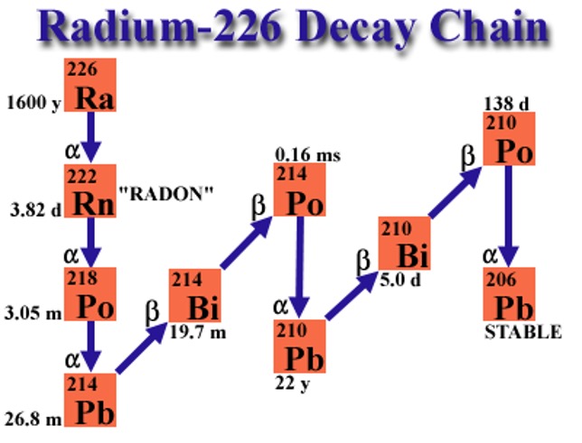
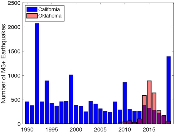
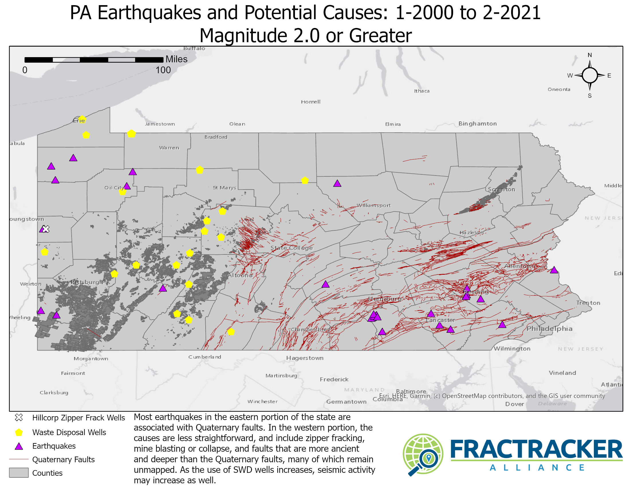

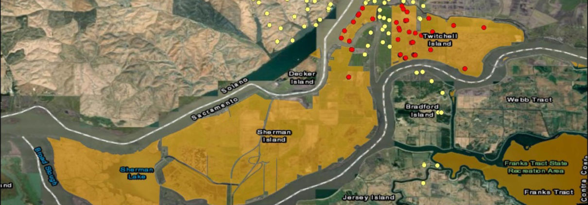
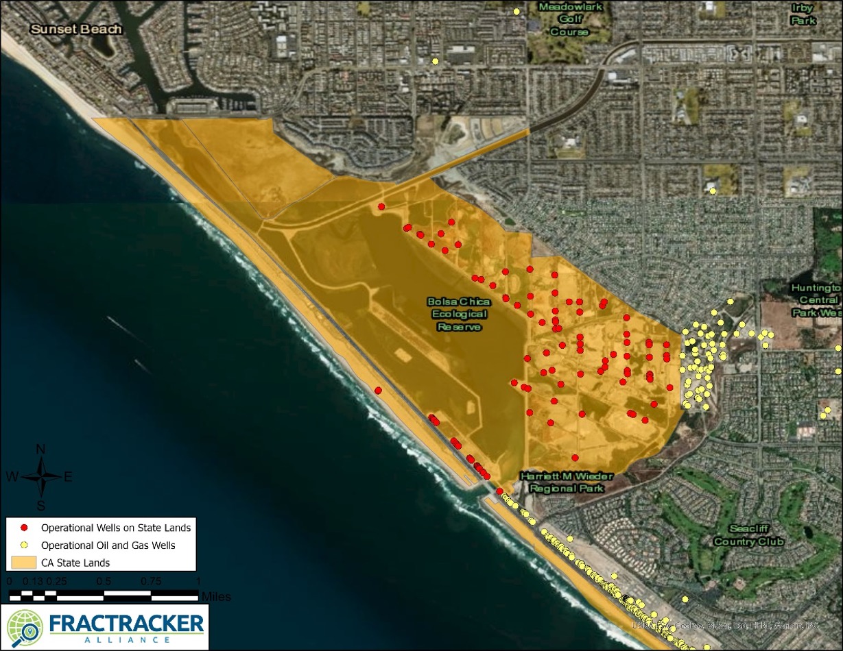
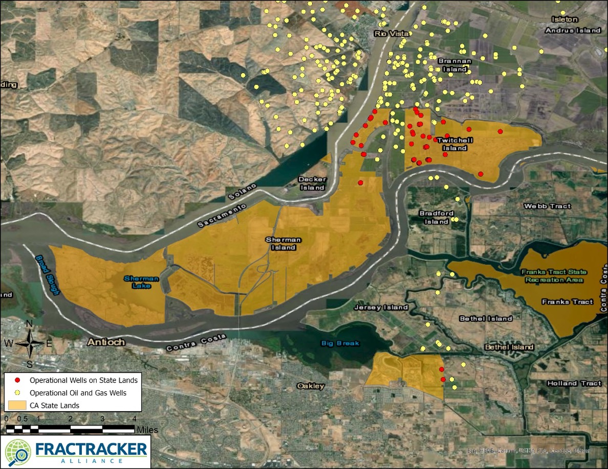


")