The majority of FracTracker’s posts are generally considered articles. These may include analysis around data, embedded maps, summaries of partner collaborations, highlights of a publication or project, guest posts, etc.
Update: The Indiegogo crowdfunding campaign for this initiative ended on August 20, 2014
An International Expedition to Address the Perils of Oil & Gas Extraction
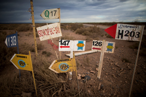
Signs point to exploration areas in the Vaca Muerta, or Dead Cow, a field in the Patagonian desert where Chevron is currently drilling fracking exploratory wells. (Photo by NY Times)
People in Argentina are concerned about fracking increasing in their country. They are aware of the impacts to people’s health and the environment that oil and gas fracking has caused – spills, leaks and explosions; air and water pollution; nausea, headaches and other health problems from toxic exposure; destruction of forests and parklands; increased earthquake risks.
They want to know the truth from those who have lived and worked near oil and gas operations in the U.S. Argentina sin Fracking has invited Earthworks, FracTracker Alliance and Ecologic Institute to come to Argentina to tell the real story.
To help fund this initiative, we have launched an Indiegogo campaign. Your contributions will make it possible for experts from these 3 American organizations to travel to Argentina, and share their experiences from the U.S. with fracking. We’ll hold several workshops in Buenos Aires and other affected communities, such as the Vaca Muerta region, where fracking is already occurring, and visit others who face the potential dangers of fracking.
With your help, we can help Argentina avoid making the mistakes that we’ve made in the U.S., and we can connect Argentinians to a new international network of environmental groups fighting fossil fuel development worldwide.
https://www.fractracker.org/a5ej20sjfwe/wp-content/uploads/2014/07/Oil-and-Gas-signs-NY-Times.jpg400600FracTracker Alliancehttps://www.fractracker.org/a5ej20sjfwe/wp-content/uploads/2025/09/2025-Wordmark-Logo.pngFracTracker Alliance2014-07-21 09:00:482020-07-21 10:42:41In Solidarity With Argentina
State Senator Joseph Scarnati III, from north-central Pennsylvania, has introduced a bill that would redefine the distinction between conventional and unconventional oil and gas wells throughout the state. In Section 1 of the bill, the sponsors try to establish the purpose of the legislation, making the case that:
Conventional oil and gas development has a benign impact on the Commonwealth
Many of the wells currently classified as conventional are developed by small businesses
Oil and gas regulations, “must permit the optimal development of oil and gas resources,” as well as protect the citizens and environment.
Previous legislation already does, and should, treat conventional and unconventional wells differently
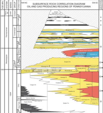
This diagram shows geologic stata in Pennsylvania. The Elk Group is between the Huron and Rhinestreet shale deposits from the Upper Devonian period. Click on the image to see the full version. Source: DCNR
Certainly, robust debate surrounds each of these points, but they are introductory in nature, not the meat and potatoes of Senate Bill 1378. What this bill does is re-categorize some of the state’s unconventional wells to the less restrictive conventional category, including:
All oil wells
All natural gas wells not drilled in shale formations
All shale wells above (shallower than) the base of the Elk Group or equivalent
All shale wells below the Elk Group from a formation that can be economically drilled without the use of hydraulic fracturing or multi-lateral bore holes
All wells drilled into any formation where the purpose is not production, including waste disposal and other injection wells
The current distinction is in fact muddled, with one DEP source indicating that the difference is entirely due to whether or not the formation being drilled into is above or below the Elk Group, and another DEP source indicates that the difference is much more nuanced, and really depends on whether the volumes of hydraulic fracturing fluid required to profitably drill into a given formation are generally high or low.
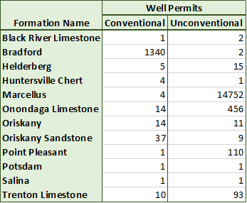
This table shows the number of distinct wells in each producing formation in Pennsylvania that has both conventional and unconventional wells drilled into it. Data source: DEP, downloaded 7/9/2014.
As one might expect, this ambiguity is represented in the data. The chart at the left shows the number of distinct number of wells by formation, for each producing formation that has both conventional and unconventional wells in the dataset. Certainly, there could be some data entry errors involved, as the vast majority of Bradford wells are conventional, and almost all of the Marcellus wells are unconventional. But there seems to be some real confusion with regards to the Oriskany, for example, which is not only deeper than the Elk Group, but the Marcellus formation as well.
While an adjustment to the distinction of conventional and unconventional wells in Pennsylvania is called for, one wonders if the definitions proposed in SB 1378 is the right way to handle it. If the idea of separating the two is based on the relative impact of the drilling operation, then a much more straightforward metric might be useful, such as providing a cutoff in the amount of hydraulic fracturing fluid used to drill a well. Further, each of the five parts of the proposed definition serve to make the definition of unconventional wells less inclusive, meaning that additional wells would be subject to the less stringent regulations, and that the state would collect less money from the impact fees that were a part of Act 13 of 2012.
Instead, it is worth checking to see whether the definition of unconventional is inclusive enough. In May of this year, FracTracker posted a blog about conventional wells that were drilled horizontally in Pennsylvania.
Conventional, non-vertical wells in Pennsylvania. Please click the expanding arrows icon at the top-right corner to access the legend and other map controls. Please zoom in to access data for each location.
These wells require large amounts of hydraulic fracturing fluids, and are already being drilled at depths of only 3,000 feet, and could go as shallow as 1,000 feet. It’s pretty easy to argue that due to the shallow nature of the wells, and the close proximity to drinking water aquifers, these wells are deserving of even more rigorous scrutiny than those drilled into the Marcellus Shale, which generally ranges from 5,000 to 9,000 feet deep throughout the state.
A summary of the different regulations regarding conventional and unconventional wells can be found from PennFuture. In general, unconventional wells must be further away from water sources and structures than their conventional counterparts, and the radius of presumptive liability for the contamination of water supplies is 2,500 feet instead of 1,000.
SB 1378 has been re-referred to the Appropriations Committee.
https://www.fractracker.org/a5ej20sjfwe/wp-content/uploads/2014/07/formations_ConUnc_07092014.png286347Matt Kelso, BAhttps://www.fractracker.org/a5ej20sjfwe/wp-content/uploads/2025/09/2025-Wordmark-Logo.pngMatt Kelso, BA2014-07-09 15:04:362020-07-21 10:42:41What’s in PA Senate Bill 1378?
By Ted Auch, OH Program Coordinator, FracTracker Alliance
Both Ohio and West Virginia citizens are concerned about the increasing shale exploration in their area and how it affects water quality. Those concerned about the drilling tend to focus on the large quantities of water required to hydraulically fracture – or “frack” – Utica and Marcellus wells. Meanwhile those concerned with water quality cite increases in truck traffic and related spills. Concerns also exist regarding the large volumes of fracking waste injected into Class II Salt Water Disposal (SWD) wells primarily located in/adjacent to Ohio’s Muskingum River Watershed.
Injection Wells & Water Usage
While Pennsylvania and WV have drilled heavily into their various shale plays, OH has seen a dramatic increase in Class II Injection wells. In 2010 OH hosted 151 injection wells, which received 50.1 Million Gallons (MGs) per quarter in total – or 331,982 gallons per well. Now, this area has 1941 injection wells accepting 937.5 MGs in total and an average of 4.3 MGs per well.
In the second quarter of 2010 the Top 10 Class II wells by volume accounted for 45.87% of total fracking waste injected in the state. Fast forward to today, the Top 10 wells account for 38.87% of the waste injected. This means that the industry and OH Department of Natural Resources Underground Injection Control (ODNR UIC) are relying on 128% more wells to handle the 1,671% increase in the fracking waste stream coming from inside OH, WV, and PA. During the same time period, freshwater usage by the directional drilling industry has increased by 261% in WV and 162% in OH.
Quantity of Disposed Waste
With respect to OH’s injection waste story there appear to be a couple of distinct trends with the following injection wells:
— Long Run Disposal #8 in Washington and Myers in Portage counties. The changes reflect a nearly exponential increase in the amount of oil and gas waste being injected, with projected quarterly increases of 6.78 and 5.64 MGs. This trend is followed by slightly less dramatic increases at several other sites: the Devco Unit #11 is up 4.81 MGs per quarter (MGPQ).
— Groselle #2 is increasing at 4.21 MGPQ, and Ohio Oil Gathering Corp II #6 is the same with an increase of 4.03 MGPQ.
— Another group of wells with similar waste statistics is the trio of the Newell Run Disposal #10 (↑2.81 MGPQ), Pander R & P #15 (↑3.23 MGPQ), and Dietrich PH (↑2.53 MGPQ).
— The final grouping are of wells that came online between the fall of 2012 and the spring of 2013 and have rapidly begun to constitute a sizeable share of the fracking waste stream. The two wells that fall within this category and rank in the Top 10 are the Adams #10 and Warren Drilling Co. #6 wells, which are experiencing quarterly increases of 3.49 and 2.41 MGs (Figure 2).
Disposal of Out-of-State Waste
These Top 10 wells also break down into groups based on the degree to which they have, are, and plan to rely on out-of-state fracking waste (Figure 3). Five wells that have continuously received more than 70% of their wastestream from out-of-state are the Newell Run Disposal (94.4), Long Run Disposal (94.7%), Ohio Oil Gathering Corp (94.2%), Groselle (94.3%), and Myers (77.2%). This group is followed by a set of three wells that reflect those that relied on out-of-state waste for 17-30% of their inputs during the early stages of Utica Shale development in OH but shifted significantly to out-of-state shale waste for ≥40% of their inputs. (More than 80% of Pander R & P’s waste stream was from out-of-state waste streams, up from ≈20% during the Fall/Winter of 2010-11). Finally, there are the Adams and Warren Drilling Co. wells, which – in addition to coming online only recently – initially heavily received out-of-state fracking waste to the tune of ≥75% but this reliance declined significantly by 51% and 26% in the case of the Adams and Warren Drilling Co. wells, respectively. This indicates that demand-side pressures are growing in Ohio and for individual Class II owners – or – the expanding Stallion Oilfield Services (which is rapidly buying up Class II wells) is responding to an exponential increase in fracking brine waste internally.
Waste Sources
We know anecdotally that much of the waste coming into OH is coming from neighboring WV and PA, which is why we are now looking into directional well water usage in these two states. WV and PA have far fewer Class II wells relative to OH and well permitting has not increased significantly there. Here in Ohio we are experiencing not just an increase in injection waste volumes but also a steady increase in water usage. The average Utica well currently utilizes 6.5-8.1 million gallons of fresh water, up from 4.6-5.3 MGs during the Fall/Winter of 2010-11 (Figure 4). Put another way, water usage is increasing on a quarterly basis by 221-333K gallons per well2. Unfortunately, this increase coincides with an increase in the reliance on freshwater (+00.42% PQ) and parallel decline in recycled water (-00.54% PQ). In addition to declining in nominal terms, recycling rates are also declining in real terms given that the rate is a percentage of an ever-increasing volume. Currently the use of freshwater and recycled water account for 6.1 MGs and 0.33 MGs per well, respectively. Given the difference in freshwater and recycled water it appears there is an average 8,319 gallon unknown fluid void per well. The quality of the water used to fill the void is important from a watershed (or drinking water) perspective. The chemicals used in the process tend to be resistant to bio-degradation and can negatively influence the chemistry of freshwater.
WV Data
WV is experiencing similar increases in water usage for their directionally drilled wells; the average well currently utilizes 7.0-9.6 MGs of fresh water – up from 2.9-5.0 MGs during the Fall/Winter of 2010-11 (↑208%). This change translates into a quarterly increase in the range of 189-353K gallons per well3. The increase coincides with an increase in the reliance on freshwater (+00.34% PQ) and related decline in recycled water (-00.67% PQ). Currently, freshwater and recycled water account for 7.7 MGs and 0.61 MGs per well, respectively. Given the difference in freshwater and recycled water, there is an average of 22,750 gallons of unaccounted for fluids being filled by unknown or proprietary fluids (Figure 5).
Figure 1. Ohio Class II Number and Volumes in 2010 and 2014
Figure 2. Quarterly volumes accepted by Ohio’s Top Ten Class II Injection Wells with respect to hydraulic fracturing brine waste.
Figure 3. Ohio’s Top Ten Class II Injection Wells w/respect to hydraulic fracturing brine waste.
Figure 4. Total water usage per Utica well and recycled Vs freshwater percentage change across Ohio’s Utica Shale wells on a quarterly basis. Data are presented quarterly (Ave. Q3-2010 to Q2-2014)
Figure 5. Changes in WV water usage for horizontally/hydraulically fractured wells w/respect to recycled water (volume & percentages) & freshwater. Data are presented quarterly (Ave. Q3-2010 to Q2-2014)
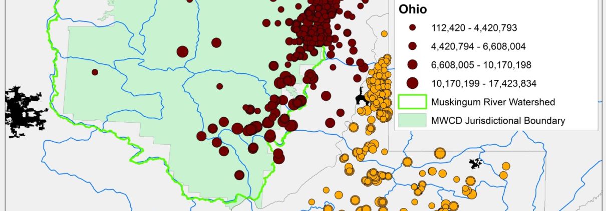
Figure 6. Unconventional drilling well water usage in OH (n = 516) and WV (n = 581) (Note: blue borders describe primary Hydrological Units w/the green outline depicting the Muskingum River watershed in OH).
The large range depends on whether you start your analysis at Q3-2010 or the aforementioned statistically robust Q3-2011.
The large range depends on whether you start your analysis at Q3-2010 or the more statistically robust Q3-2011.
MWCD water sales approved to date: 1) Seneca Lake for Antero: 15 million gallons at 1.5mm per day, 2) Piedmont Lake for Gulfport: 45 million gallons at 2 million per day, 3) Clendening for American Energy Utica: 60 million gallons at 2 million per day.
https://www.fractracker.org/a5ej20sjfwe/wp-content/uploads/2014/06/OH_WV_Water.jpg11051427Ted Auch, PhDhttps://www.fractracker.org/a5ej20sjfwe/wp-content/uploads/2025/09/2025-Wordmark-Logo.pngTed Auch, PhD2014-07-03 14:26:532020-07-21 10:42:40OH and WV Shale Gas Water Usage and Waste Injection
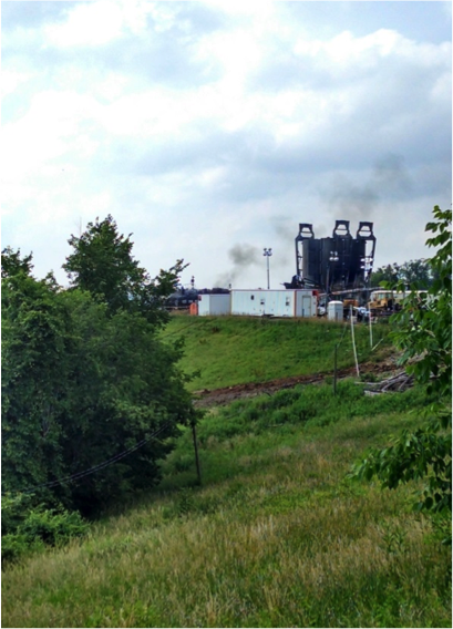
A First-hand Look at the Recent Statoil Well Pad Fire
By Evan Collins and Rachel Wadell, Summer Research Interns, Wheeling Jesuit University
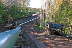
Monroe Co. Ohio – Site of June 2014 Statoil well pad fire
After sitting in the non-air-conditioned lab on a muggy Monday afternoon (June 30, 2014), we were more than ready to go for a ride to Opossum Creek after our professor at Wheeling Jesuit University mentioned a field work opportunity. As a researcher concerned about drilling’s impacts, our professor has given many talks on the damaging effects that unconventional drilling can have on the local ecosystem. During the trip down route 7, he explained that there had been a serious incident on a well pad in Monroe County, Ohio (along the OH-WV border) on Saturday morning.
About the Incident
Hydraulic tubing had caught fire at Statoil’s Eisenbarth well pad, resulting in the evacuation of 20-25 nearby residents.1 Statoil North America is a relatively large Norwegian-based company, employing roughly 23,000 workers, that operates all of its OH shale wells in Monroe County.2 The Eisenbarth pad has 8 wells, 2 of which are active.1 However, the fire did not result from operations underground. All burning occurred at the surface from faulty hydraulic lines.
Resulting Fish Kill?
Several fish from the reported fish kill of Opossum Creek in the wake of the recent well pad fire in Monroe County, OH.
When we arrived at Opossum Creek, which flows into the Ohio River north of New Martinsville, WV, it smelled like the fresh scent of lemon pine-sol. A quick look revealed that there was definitely something wrong with the water. The water had an orange tint, aquatic plants were wilting, and dozens of fish were belly-up. In several shallow pools along the creek, a few small mouth bass were still alive, but they appeared to be disoriented. As we drove down the rocky path towards the upstream contamination site, we passed other water samplers. One group was from the Center for Toxicology and Environmental Health (CTEH). The consulting firm was sampling for volatile organic compounds, while we were looking for the presence of halogens such as Bromide and Chloride. These are the precursors to trihalomethanes, a known environmental toxicant.
Visiting the Site
After collecting water samples, we decided to visit the site of the fire. As we drove up the ridge, we passed another active well site. Pausing for a break and a peek at the well, we gazed upon the scenic Appalachian hillsides and enjoyed the peaceful drone of the well site. Further up the road, we came to the skeletal frame of the previous Statoil site. Workers and members of consulting agencies, such as CTEH, surrounded the still smoking debris. After taking a few pictures, we ran into a woman who lived just a half-mile from the well site. We asked her about the fire and she stated that she did not appreciate having to evacuate her home. Surrounding plants and animals were not able to be evacuated, however.
Somehow the fish living in Opossum Creek, just downhill from the well, ended up dead after the fire. The topography of the area suggests that runoff from the well would likely flow in a different direction, so the direct cause of the fish kill is still obscure. While it is possible that chemicals used on the well pad ran into the creek while the fire was being extinguished, the OH Department of Natural Resources “can’t confirm if it (the fish kill) is related to the gas-well fire.”3 In reference to the fire, a local resident said “It’s one of those things that happens. My God, they’re 20,000 feet down in the ground. Fracking isn’t going to hurt anything around here. The real danger is this kind of thing — fire or accidents like that.”4
Lacking Transparency
Run by Statoil North America, Eisenbarth well pad in Monroe County, Ohio is still smoking after the fire.
Unfortunately, this sentiment is just another example of the general public being ill-informed about all of the aspects involved in unconventional drilling. This knowledge gap is largely due to the fact that oil and gas extraction companies are not always transparent about their operations or the risks of drilling. In addition to the potential for water pollution, earthquakes, and illness due to chemicals, air pollution from active unconventional well sites is increasing annually.
CO2 Emissions
Using prior years’ data, from 2010 to 2013, we determined that the average CO2 output from unconventional gas wells in 2013 was equal to that of an average coal-fired plant. If growth continued at this rate, the total emissions of all unconventional wells in West Virginia will approximate 10 coal-fired power plants in the year 2030. Coincidentally, this is the same year which the EPA has mandated a 30 percent reduction in CO2 emissions by all current forms of energy production. However, recent reports suggest that the amount of exported gas will quadruple by 2030, meaning that the growth will actually be larger than originally predicted.5 Yet, this number only includes the CO2 produced during extraction. It does not include the CO2 released when the natural gas is burned, or the gas that escapes from leaks in the wells.
Long-Term Impacts
Fires and explosions are just some of the dangers involved in unconventional drilling. While they can be immediately damaging, it is important to look at the long-term impacts that this industry has on the environment. Over time, seepage into drinking water wells and aquifers from underground injection sites will contaminate these potable sources of water. Constant drilling has also led to the occurrence of unnatural earthquakes. CO2 emissions, if left unchecked, could easily eclipse the output from coal-fired power plants – meaning that modern natural gas drilling isn’t necessarily the “clean alternative” as it has been advertised.
https://www.fractracker.org/a5ej20sjfwe/wp-content/uploads/2014/07/FishKillOH2014-PhotobyEvan-CollinsRachelWadell.png569425FracTracker Alliancehttps://www.fractracker.org/a5ej20sjfwe/wp-content/uploads/2025/09/2025-Wordmark-Logo.pngFracTracker Alliance2014-07-03 10:22:222020-07-21 10:42:28These Fish Weren’t Playing Opossum (Creek)
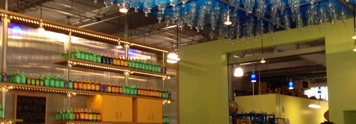
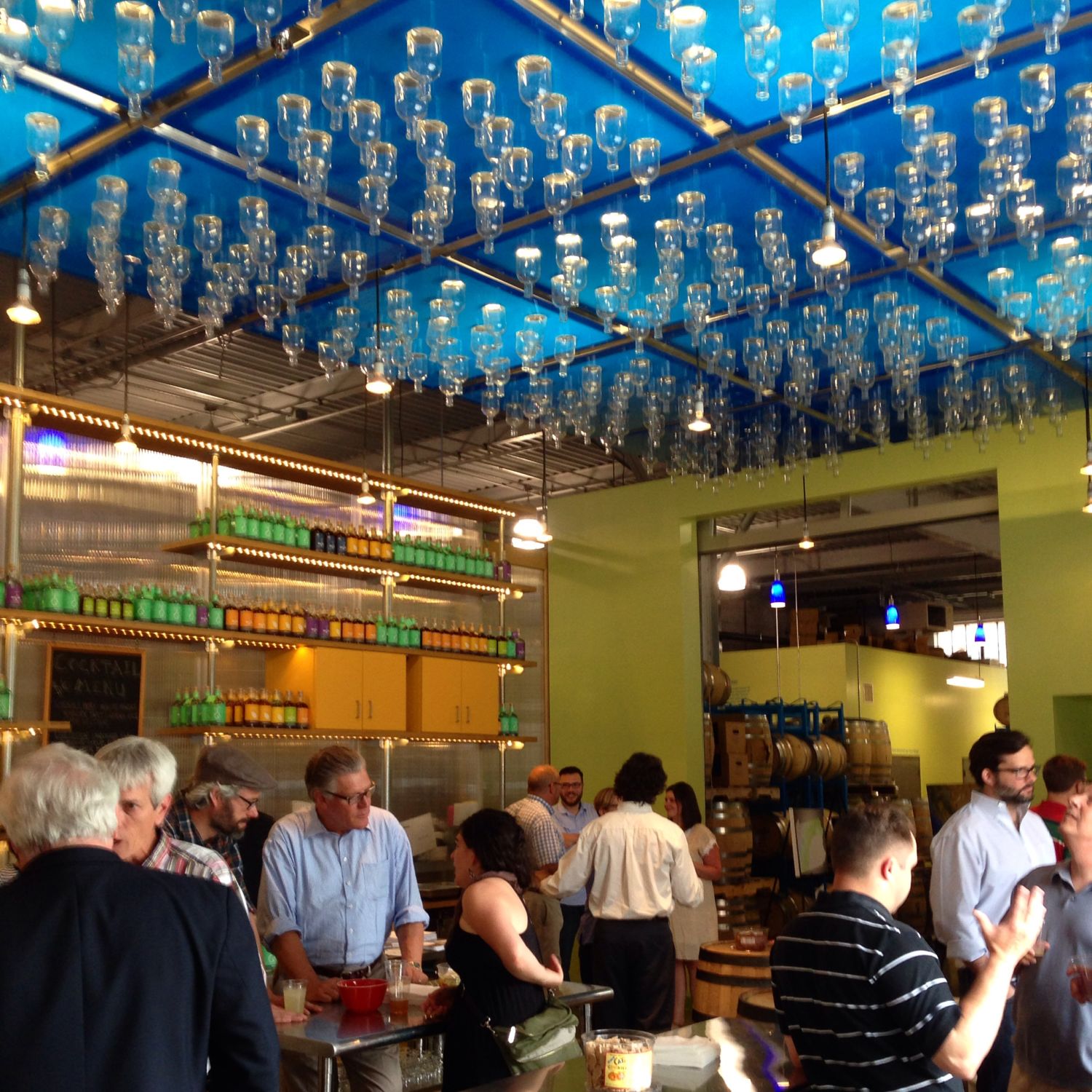
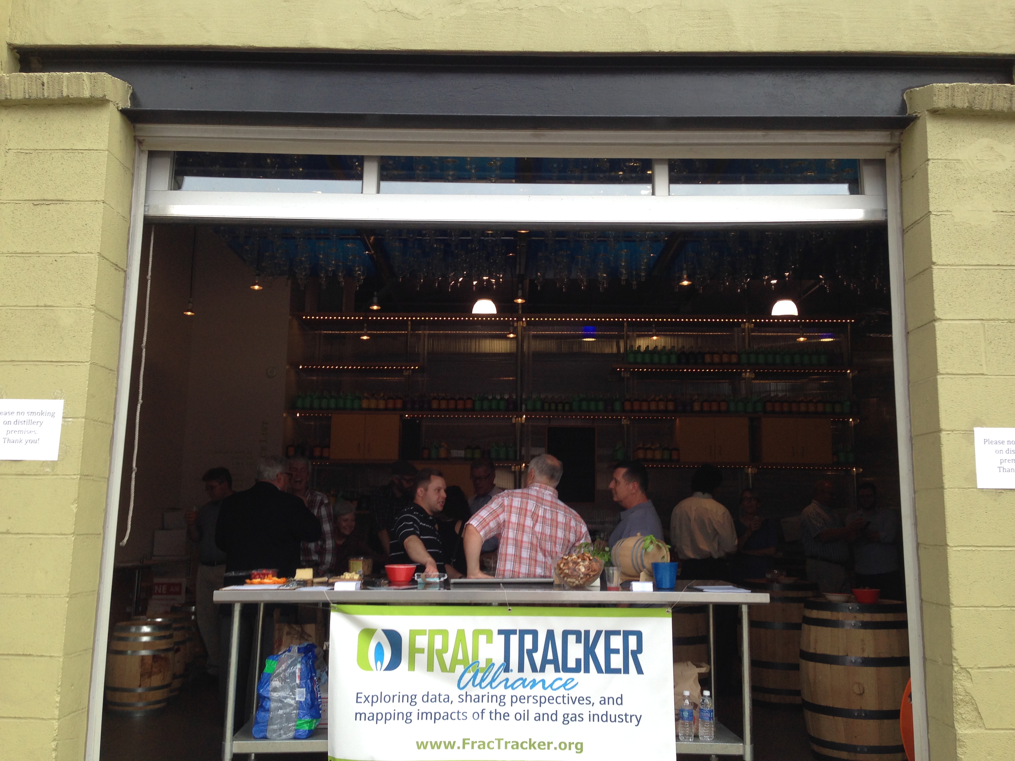
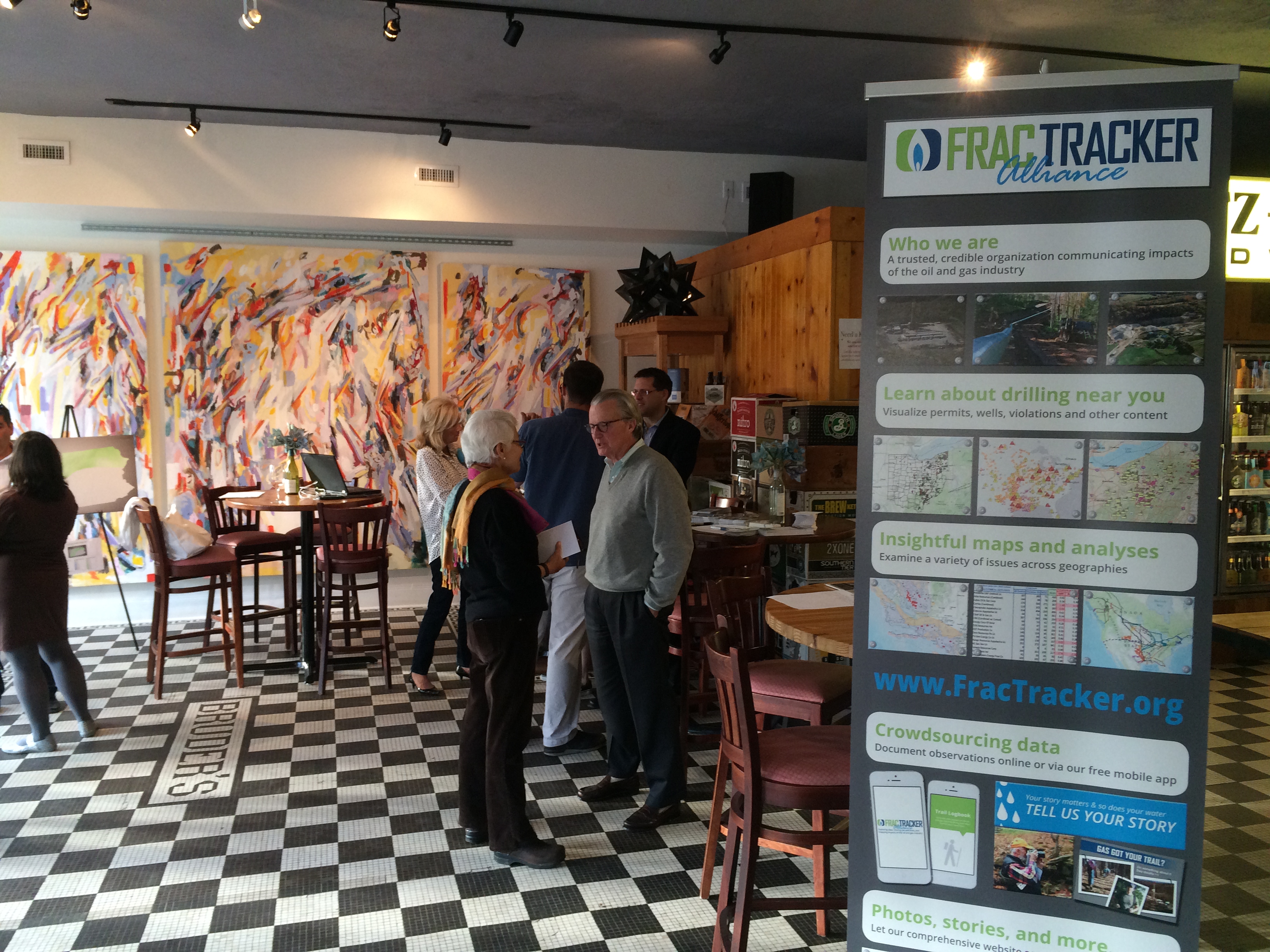
By Brook Lenker, Executive Director, FracTracker Alliance
Enjoying some whiskey in Pittsburgh
It’s almost July, but just a few weeks ago, FracTracker wrapped up the last of three fundraising events. From a site in San Francisco overlooking the Pacific to a budding distillery in Pittsburgh’s Strip District, friends and colleagues came together to show their support for our work and their concern about the effects of unconventional drilling. If you were able to join us for these events – whatever the motivation, we appreciated your collective, deliberate act of kindness. Thank you!
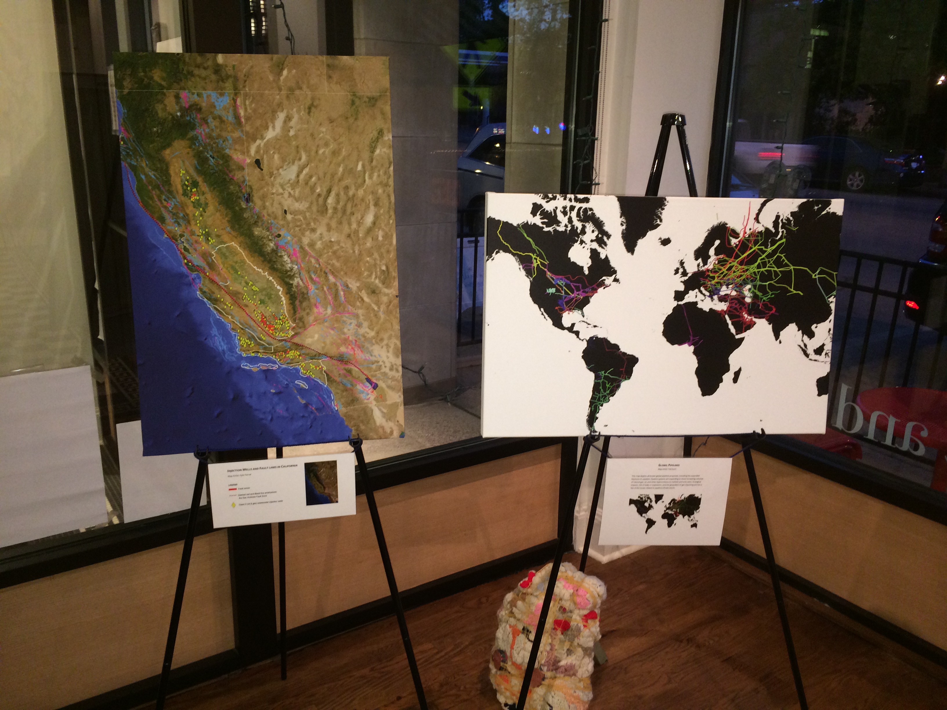
The gatherings were generally small but lots of fun – full of conversation, positive energy, and, yes, good spirits. At the Cleveland Heights event, we even had live music thanks to the jazzy guitar of Alan Brooks and at all three venues a colorful exhibit of thought-provoking, conversation-stoking maps entitled “Cartography on Canvas.” These events were our first foray into fundraisers. From the experience they’ll be improved and made even more memorable, unique, extraordinary. That’s our goal.
We aim to entice more attendees, enhance our revenue, and, most importantly, grow the network of the informed – not just informed about the activities of FracTracker but of all the groups, efforts, and learnings related to the impacts of extreme hydrocarbon extraction. Soon, another round of events – guaranteed to be mood improving, mind expanding affairs – will be rolled out. Prepare to mark your calendars, join the fun, and make your own social statement!
A special thank you goes out to FracTracker staff, interns, and board members who put in extra time and effort to help ensure the success of these initial fundraisers. Thank you, too, to our incredible door prize and auction item contributors:
https://www.fractracker.org/a5ej20sjfwe/wp-content/uploads/2014/06/IMG_6508.jpg15001500FracTracker Alliancehttps://www.fractracker.org/a5ej20sjfwe/wp-content/uploads/2025/09/2025-Wordmark-Logo.pngFracTracker Alliance2014-06-30 11:08:202020-07-21 10:42:28Putting the “Fun” in Fundraisers
By Jill Terner, PA Communications Intern, FracTracker Alliance
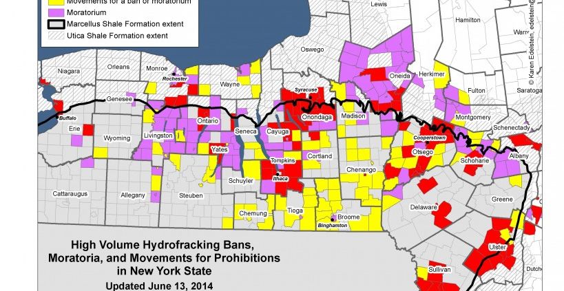
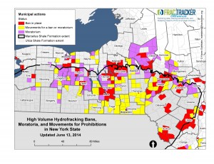
There are strong public opinions in some cases related to unconventional drilling. This map shows municipal movements in NY State against the process (06/13/2014)
In the previous two installments of this three part series, I discussed how sustainability provides a common platform for people who support and deny the use of hydraulic fracturing to extract oil and natural gas from the ground. While these opposing sides may frequently use sustainability in their rhetoric, the term has different connotations depending on which side is presented. The dynamic definition of sustainability makes it a boundary object, or a term that many people can use in shared discourse, all while defining it in different nuanced ways1. This way, the definition of sustainability alters between groups of people, and may also change over time.
First, I wrote about how pro-industry groups tend to focus primarily on the economic angle of sustainability rather than a more holistic understanding when arguing that hydraulic fracturing is the best choice for local and national communities. In my second post, I discussed how pro-environment groups see sustainability as a multifaceted entity, treating social and environmental sustainability with as much importance as economic. Here, I will focus on what can cause differences in public perceptions of hydraulic fracturing, as well as what might be done to mitigate potential confusion caused by competing definitions of sustainability.
A Few Explanations for Differing Opinions
A national survey conducted in 2013 found that by and large, people had no opinion of hydraulic fracturing. This was probably due to the fact that the majority of respondents indicated that they had heard little to nothing about hydraulic fracturing also known as unconventional drilling. Those who did identify as having an opinion either for or against drilling were split nearly evenly*. While survey participants on both sides recognized that there could be several economic benefits related to industrial presence, they also acknowledged that distribution of these benefits might not be equitable. Additionally, recognition of environmental and social threats is correlated with a negative view of industry. The stronger a respondents’ concern is about damaging environmental and social outcomes resulting from drilling activities, the more likely they were to express negative opinions about the industry2.
What is responsible for this difference of opinion? One possible explanation lies in the level of drilling activity a given community is experiencing. In areas where hydraulic fracturing is more prevalent, residents are more likely to have leased their land to drilling companies, so they are more likely to adjust their attitude to reflect their actions. They have made a significant investment by leasing their land, so they are likely to be optimistic about the payoff3.
Relatedly, the length of time that industry has been active in an area might also affect public perceptions. When industry is relatively new, many residents of nearby communities are optimistic about the economic gains that it may bring. However, alongside this optimism, residents may also express trepidation regarding what the influx of new people and wealth might do to community integrity. Over time, though, residents of areas where industry has maintained a continued presence may have adjusted to the changes brought on by industry, or have had their initial fears mitigated3, 4,5.
Geographically speaking, proximity to a major metropolitan area may also play a role in public perception of unconventional drilling. In counties where there are more metropolitan areas, there is the potential for an increase in negative social side effects. For example, an increase in violent crimes5, 6, uneven distribution of wealth generated by industry4, and loss of community character4, 6, might be offset by the fact that the influx of new workers makes up a smaller proportion of the county population than in less urbanized counties4.
On a broader geographical scale, state-by-state differences in opinion could be largely due to how prohibitive or permissive laws are regarding drilling. In states such as New York, where legislation demonstrates concern for the environment and safety, residents may be more likely to see sustainability as something more than just economic. On the other hand, in states like Pennsylvania where legislation is relatively permissive, residents may be more likely to see economic sustainability as most important due to the political climate4. This view is also known as the chicken/egg phenomenon: does the public’s opinion sway legislation, or does legislation drive public opinion? Either way, the differences across state lines remains.
What can be done to better inform public opinion?
Above, I mentioned a study where researchers found that the vast majority of survey participants held no opinion regarding unconventional drilling, largely due to lack of knowledge about it2. Therefore making unbiased information readily available and understandable to the public will allow them to make informed opinions on the subject. For example, having access to objective literature regarding unconventional drilling provides the opportunity to increase awareness and inform individuals about the practice of hydraulic fracturing and its potential impacts. In order to have the most impact we must first asses where gaps in public knowledge lie. Engaging in projects such as community based participatory research and then qualitatively assessing the results will reveal common misconceptions or knowledge gaps that need to be addressed through educational programs.
Also, most predictions regarding the unconventional drilling boom are based on a boom-and-bust cycles of past industries4. For example, they look at longitudinal studies where representative groups of residents within communities are followed over time, and they also focus on existing communities affected by industry identifying the social, environmental, and economic outcomes related to industry. This way, any comparisons drawn would be within the same industry, even if they were between two different cities.
Finally, the information gleaned from community based participatory or longitudinal research should be presented by an unbiased party and made easily available. Promoting transparency within biased institutions is equally important. While each entity uses the term “sustainability” to dynamically fit its rhetorical needs, few entities prioritize the same kinds of sustainability. Therefore, it is up to industry, environmental groups, and independent researchers alike to provide a transparent atmosphere of honest information so that individuals can decide which understanding of sustainability they would like to see informing the progress of unconventional drilling in their communities.
About the Author
Jill Terner is an MPH candidate at Columbia University’s Mailman School of Public Health and a native Pittsburgher. Interning with FracTracker in fall of 2013 has cemented Jill’s interest in combining Environmental Public Health with her passion for Social Justice. After completing her MPH in May 2015, Jill hopes to find work helping people better understand, interact with, and mitigate threats to their environment – and how their environment impacts their health.
Footnotes
* 13% did not know how much they had heard about drilling, 39% had heard nothing at all, 16% had heard “a little”, 22% had heard “some”, and 9% had heard “a lot.” Of these respondents, 58% did not know/were undecided about whether they supported drilling, 20% were opposed, and 22% were supportive2.
Sources
Star, S. L., & Griesemer, J. R. (1989). Institutional ecology, ‘translations’ and boundary objects: Amateurs and professionals in Berkeley’s museum of vertebrate zoology, 1907-39. Social Studies of Science, 19, 387-420.
Boudet, H., Carke, C., Bugden, D., Maibach, E., Roser-Renouf, C., & Leiserowitz, A. (2013). “fracking” controversy and communication: Using national survey data to understand public erceptions of hydraulic fracturing. Energy Policy, 65, 57-67.
Kriesky, J., Goldstein, B. D., Zell, K., & Beach, S. (2013). Differing opinions about natural gas drillingin two adjacent counties with different livels of drilling activity. Energy Policy, 50, 228-236.
Wynveen, B. J. (2011). A thematic analysis of local respondents’ perceptions of barnett shale energy development. Journal of Rural Social Sciences, 26(1), 8-31.
Brasier, K. J., Filteau, M. R., McLaughlin, D. K., Jacquet, J., Stedman, R. C., Kelsey, T. W., & Goetz, S. J. (2011). Residents’ perceptions of community and environmental impacts from development of natural gas in the Marcellus Shale: A comparison of Pennsylvania and New York cases. Journal of Rural Social Sciences, 26(1), 32-61.
Korfmacher, K. S., Jones, W. A., Malone, S. L., & Vinci, L. F. (2013). Public Health and High Volume Hydraulic Fracturing. New Solutions, 23(1) 13-31.
https://www.fractracker.org/a5ej20sjfwe/wp-content/uploads/2012/04/municipal_movements_against_rev06-132014_MAP-e1402678058310.jpg633819FracTracker Alliancehttps://www.fractracker.org/a5ej20sjfwe/wp-content/uploads/2025/09/2025-Wordmark-Logo.pngFracTracker Alliance2014-06-25 12:51:542020-07-21 10:42:28Public Perception of Sustainability
By Karen Edelstein, NY Program Coordinator, FracTracker Alliance
Background
Over the past month and a half, a new pipeline controversy has been stirring in Pennsylvania. The proposed $2 billion “Central Penn Pipeline” will be built to carry shale gas throughout the country. Starting in Susquehanna County, the 178 mile pipeline will run through Lebanon and Lancaster counties to connect the existing Tennessee Pipeline in the north with the Transco Pipeline in the south.
Oklahoma-based Williams Partners, the company proposing the pipeline, says that the project would help move gas from PA to locations as far south as Georgia and Alabama, in addition to adding relief from higher energy bills. The “Atlantic Sunrise Project,” as it is formally known, would also require the construction of two new 30,000 horse-power compressor stations: “Station 605” along the northern leg of the pipeline in Susquehanna County, as well as “Station 610” on the southern part of the pipeline. The northern part of the proposed pipeline will be 30 inches in diameter and run for about 56 miles; the southern portion will be 42 inches in diameter and about 122 miles long.
According to the US Energy Information Agency (EIA), in 2008, PA had over 8,700 miles of pipeline. Since then, that figure has increased significantly as the shale plays in PA continue to be exploited. Industry maintains that pipelines are the safest method for moving gas from the well to market, and has noted that for safety concerns they have intentionally co-located 36% of the northern part of the pipeline within the rights-of-way of Transco’s or other utility’s pipelines.
Despite the sanguine view of this project by industry, residents have rallied against the pipeline since mid-April, when landowners started getting information packets in the mail about the proposal.
Pipeline Proposal Map
While the exact route of the pipeline has yet to be determined, FracTracker has adapted documents from Oklahoma-based Williams Partners Company to provide this interactive map below. The proposed pipeline is shown in red.
For a full-screen version of this map (with legend), click here.
Proposal Concerns
Public awareness and concern about the pipeline continues to build, as was evident when 1,100 residents attended an open house in Millersville, PA on June 10th hosted by Williams. For more information see this article in Lancaster Online.
The Lancaster County Conservancy has advocated moving the pipeline away from various sensitive habitats including the Tucquan Glen Nature Preserve, Shenk’s Ferry Wildflower Preserve, Fishing Creek, Kelly’s Run, and Rock Springs to preserve the wildlife and beauty of those areas. According to Williams:
The pipeline company must evaluate a number of environmental factors, including potential impacts on residents, threatened and endangered species, wetlands, water bodies, groundwater, fish, vegetation, wildlife, cultural resources, geology, soils, land use, air and noise quality… More
Despite what the website says, Williams admitted to not analyzing the pipeline route for possible sensitive habitat encroachment, and instead, they will simply follow the existing utility routes.
Williams, according to a report by WGAL Channel 8 in PA “relies on the communities affected to bring up any potential problems.” His statement was backed up when residents in a packed hearing room in Lancaster County voiced their opposition, resulting in Williams Partners now considering extending their pipeline by 2 ½ miles to get around the sensitive natural area at Tucquan Glen. An alternate route to avoid Shenk’s Ferry, however, had not been put forward.
Lancaster Farmland Trust is concerned about the plan for the pipeline to pass through several protected farms, and Lebanon County Commissioner Jo Ellen Litz has also taken a strong stand against the current proposed route. The proposed pipeline would not only go through farmlands, but it is also expected to cross the Appalachian Trail, Swatara State Park, and Lebanon Valley Rails to Trails.
Pipeline impacts are not limited to conservation and agriculture. There is increasing concern that the risks posed by large-diameter, high pressure pipelines such as this one may prevent nearby homeowners from keeping their mortgage loans or homeowner’s insurance. Future purchasers of the property may also encounter difficulty being approved for a mortgage loan or homeowner’s insurance.
While the pipeline company can purchase pipeline easements from property owners, industry can also petition the government to take the land by eminent domain from unwilling property owners. Pipeline rights-of-way acquired through eminent domain for these pipelines could potentially complicate a private property owner’s mortgage financing and homeowner’s insurance.
The final decisions about the siting of the pipeline is ultimately up to FERC, the Federal Energy Regulatory Commission.
Resources
Williams’ original maps of the pipelines can be viewed here: SOUTH | NORTH
https://www.fractracker.org/a5ej20sjfwe/wp-content/uploads/2014/06/5550c-Pipeline-Marc-1-e1403196615466.jpg200300Karen Edelsteinhttps://www.fractracker.org/a5ej20sjfwe/wp-content/uploads/2025/09/2025-Wordmark-Logo.pngKaren Edelstein2014-06-20 10:17:192020-07-21 10:42:27Central Penn Pipeline Under Debate
By Ted Auch, OH Program Coordinator, FracTracker Alliance
No matter where you live in Ohio you have probably asked yourself if crime trends will be – or have already been – affected by the shale gas boom.
To quantify the relationship between crime rates and oil and gas development, we compared 14 OH counties (that have more than 10 Utica permits) to statewide safety metrics. Ohio State Highway Patrol’s Statistical Analysis Unit provided us with the necessary crime data. From this dataset, we chose to analyze several metrics:
a. three types of arrests,
b. two types of violations and accidents, and
c. misdemeanors and suspended licenses (as proxies for changes in safety).
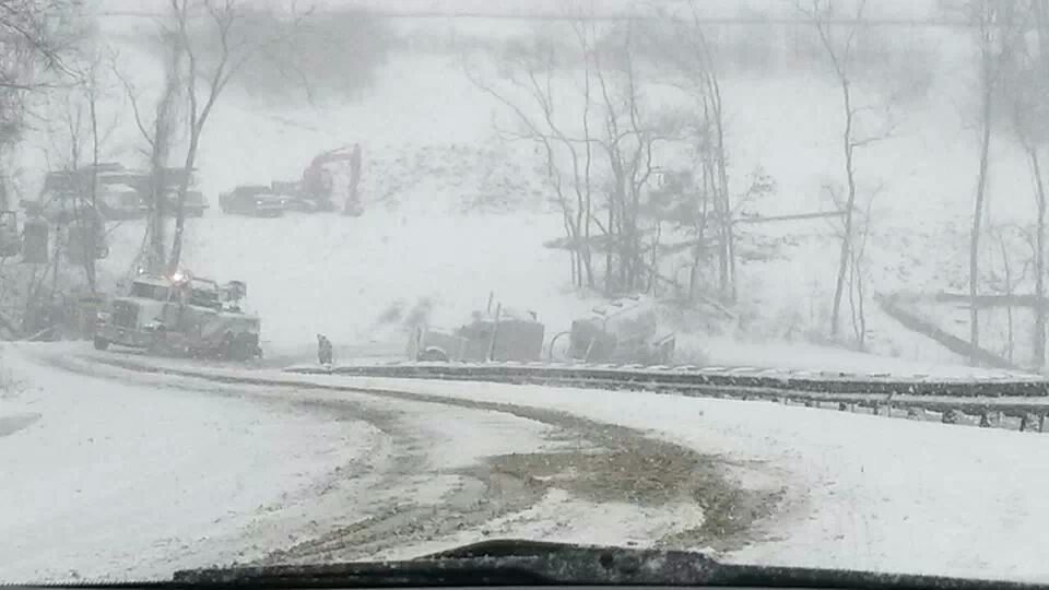
Accident involving truck carrying freshwater for fracking between Jan. 20 and 27 of 2014 during snowstorm adjacent to Seneca Lake, Noble and Guernsey Counties, OH adjacent to Antero pad off State Route 147
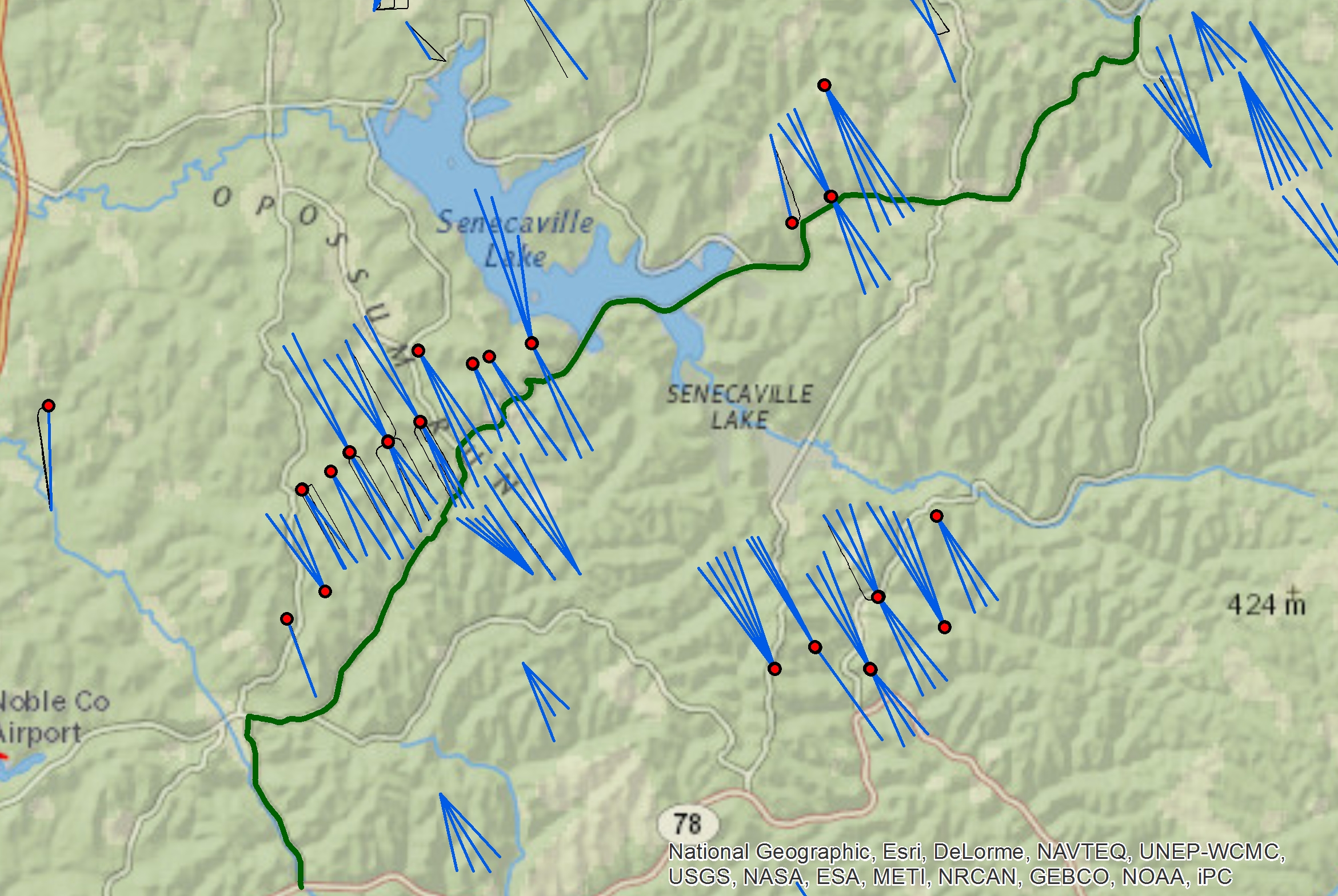
Map of Senaca Lake, OH Jan 2014 frackwater truck accident including producing or drilled Antero wells (Red Points) and laterals along with State Route 147
Crunching the Data
The data in Table 1 below are corrected for changes in population at the state level (+0.2% per year) and at the county level, with the annualized rate for the counties of interest ranging between -2.2% in Jefferson and -0.05 in Tuscarawas. We used the first four months of 2014 to determine an annualized rate for the rest of 2014. Since the first Utica permit was issued on Sept. 28, 2010, we assumed that the 2009 data would be an close measure for the ambient levels for the nine crime metrics we investigated across Ohio prior to shale gas development.
Statewide Crime Trends
Overturned frac sand trucks in Carroll County, OH May, 2014 (Courtesy of Carol McIntire, The Free Press Standard)
Commercial Vehicle Enforcements (CVE) and Crashes Investigated are the only metrics that increase by 8.9% and 6.9% per year, larger than the statewide averages of 2.8% and 6.0%. Respectively, 10 of the 14 shale gas counties have experienced rates that exceed the state average. Noble, Harrison, Columbiana, Carroll, and Monroe are experiencing annualized CVE increases that are 15-57% higher than Ohio as a whole.
Meanwhile, Crashes Investigated are increasing at a slower pace relative to the state wide average, with Carroll, Noble, and Jefferson counties experiencing >5% rate increases relative to the entire state (Table 1). There is a strong increasing linear relationship between the number of Utica permits and the average percent change in CVE and Crashes Investigated. The former accounts for a combined 66% change in the latter. From a macro perspective, the Utica counties accounted for 19.8% of all OH CVEs in 2009 prior to shale gas exploration and now account for 25.1% of all CVEs. Crashes Investigated as a percentage of state totals, however, only increased from 21.3% to 21.7%.
The other variable that is significantly and positively correlated with Utica permitting at the present time is the number of Suspended License reports, with the former explaining 22% of the average annual change in the latter since 2009.
Given that we investigated changes in nine public safety metrics we thought it would be worth categorizing the fourteen counties by state wide averages:
Significantly Less Safe (SLS) – >5 of 9 metrics increasing,
Noticeably Less Safe (NLS) – 4 metrics, and
Marginally Less Safe (MLS) – <3 metrics.
Our findings support that about half the Utica counties fall within the SLS category, with Harrison, Jefferson, Columbiana, and Trumbull experiencing higher relative rates across seven or more of the metrics investigated. Trumbell specifically has had public safety rate increases that are greater than the state in all categories but for Suspended Licenses. Guernsey and Washington counties fall within the NLS category; both are seeing elevated Resisting Arrests and CVEs relative to changes in statewide rates. Surprisingly, Carroll County, home to 404 Utica permits as of the middle of May 2014, falls within the MLS category with only two of nine metrics increasing at a rate that exceeds the state’s. However, the two metrics that are worse than the state average (Crashes Investigated (+21.4%) and CVEs (59.8%)) are increasing at a rate that is significantly higher than the other Ohio Utica counties. Additional MLS counties include Belmont, Portage, and Monroe, which are in the upper, middle, and lower third of Utica permits at the present time.
Conclusion
While correlation does not mean causation, there is a significant correlation between certain public safety metrics and Utica permitting in Ohio’s primary shale gas counties, specifically when looking at Crashes Investigated and CVEs. Additionally, many of the Ohio Utica counties are experiencing notable increases in criminal activity. Whether this trend will continue to increase in the long-term is uncertain, but the short-term trends are concerning given that these counties populations are decreasing; there is more criminal activity within a smaller population. Finally, these trends will differ based on whether or not county sheriffs and emergency responders working with the Ohio State Highway Patrol have the necessary resources and manpower to address increasing criminal activity. This issue is of concern to most southeastern Ohioans regardless of their stance on fracking. We will continue to monitor these relationships and are working to generate a map in the coming months that illustrates these trends.
Table 1. Average percent change in select public safety metrics across Ohio’s primary Utica Shale Counties relative to parallel changes across the state of Ohio between 2009 and 2014.
Percent Change Between 2009 and 2014†
Arrests
Violations
County
Felony
Resisting
OVI
Weapons
Drug
Crashes Investigated
CVE
Misdemeanor Issued
Suspended License
Noble (93, 6‡)
87.7
0
10.5
16.9
16.8
11.2
50.5
11.8
7.4
Harrison (232, 0)
22.3
0
35.8
0
34.3
10.1
34.7
67.1
33.3
Belmont (102, 2)
12.7
5.5
2.2
17.2
20.3
10.5
4.0
16.6
10.2
Jefferson (39, 1)
50.1
3.6
11.6
43.3
45.9
11.3
12.5
42.0
10.4
Columbiana (103, 0)
20.3
-3.8
6.9
28.9
27.1
7.9
17.8
25.9
10.6
Tuscarawas (16, 6)
41.2
28.9
7.0
0
0.8
7.6
12.0
61.4
3.6
Washington (10, 13)
10.1
52.7
-2.7
47.3
19.8
8.3
4.6
19.2
2.6
Stark (13, 17)
7.3
9.4
0.3
46.4
7.2
6.7
2.6
11.1
-0.5
Trumbull (15, 20)
32.9
18.9
8.6
42.9
42.1
9.3
11.5
41.1
9.4
Mahoning (30, 10)
21.4
20.7
3.6
81.4
31.8
6.0
8.5
27.7
10.2
Portage (15, 19)
80.7
4.5
4.1
85.0
40.3
3.5
1.6
15.5
7.6
Guernsey (99, 5)
22.8
32.9
8.1
14.7
10.4
2.7
11.0
10.8
7.6
Carroll (404, 4)
0
0
-20.2
0
-29.1
21.4
59.8
-30.2
3.8
Monroe (80, 0)
0
0
-4.1
0
0
97.4
50.8
20.4
27.0
County
16.5
4.3
3.5
10.3
17.6
6.9
8.9
17.8
5.8
State
17.4
6.7
7.3
16.5
23.6
6.0
2.8
24.5
10.5
% of State 2009
14.0
17.6
19.3
18.7
16.1
21.3
19.8
17.8
18.4
% of State 2014
12.9
15.2
16.7
16.8
14.0
21.7
25.1
13.1
14.5
† 2014 annualized using the first 4 months of the year.
‡ Number of Permitted Utica wells and Class II Salt Water Disposal (SWD) wells as of May, 2014
https://www.fractracker.org/a5ej20sjfwe/wp-content/uploads/2014/06/Sand-truck-rollover-for-Fractracker.jpg255432Ted Auch, PhDhttps://www.fractracker.org/a5ej20sjfwe/wp-content/uploads/2025/09/2025-Wordmark-Logo.pngTed Auch, PhD2014-06-09 14:26:222020-07-21 10:42:27Crime and the Utica Shale
By Andrew Donakowski, Northeastern Illinois University
Land cover data can play an important role in spatial analysis; satellite or aerial imagery can effectively demonstrate the extent and make-up of land cover characteristics for large areas of land. For fracking analysis, this can be used to explore important spatial relationships between fracking infrastructure and the area and/or ecosystems surrounding them. Working with FracTracker, I have compiled data concerning land cover classifications and geologic rock areas to examine areas that may be particularly vulnerable to unconventional drilling – e.g. fracking. After computing the makeup of land cover type for each geologic area, I then mapped locations of known fracking wells for further analysis. This is part of FracTracker’s ongoing interest in understanding changes in ecosystem services and plant/soil productivity associated with well pads, pipelines, retention ponds, etc.
Developed
First, by looking at the Developed areas (below), we can see that, for the most part, hydraulic fracturing is occurring relatively far from large population areas. (That is to say, on this map we can see that these types of wells are not found as often in areas where population density is high (<20 people per square mile) or a Developed land cover classification is predominate as they are in areas with a lower Develop land cover percentage). However, we can also see that there is quite a large cluster of fracking wells in the southern portion of the state, and many cities fall within 5 or 10 mi of some wells. While there may not be an immediate danger to cities that fall within this radius, we can see that some areas of the state may be more likely to encounter the effects of fracking and its associated infrastructure than others.
Forested
Next, the map depicting Forested land cover areas is, in my opinion, the most aesthetically groovy of the land cover maps; the variations in forested areas throughout the state provide a cool image. By looking at this data, we can see that much of California’s forested land lies in the northern part of the state, while most fracking wells are located in the south and central parts of the state.
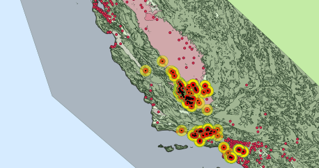
Cultivated
To me, the most interesting map is the one below showing the location of fracking wells in relation to Cultivated lands (which includes pasture areas and cropland). What is interesting to note is the fertile Central Valley, where a high percentage of land is covered with agriculture and pasture lands (Note: The Central Valley accounts for 1% of US farmland but 25% of all production by value). Notably, it is also where many fracking wells are concentrated. When one stops to think about this, it makes sense: Farmers and rural landowners are often approached with proposals to allow drilling and other non-farming activities on their land. Yet, it also raises a potential area for concern: A lot of crops grown in this area are shipped across the country to feed a significant number of people. When we consider the uncertainties of fracking on surrounding areas, we must also consider what effects fracking could have beyond the immediate area and think about how fracking could affect what is produced in that area (in this case, it is something as important as our food supply.)
The Usefulness of Maps
Finally, as previously mentioned, mapping the extent of these land coverage can be useful for future analysis. Knowing now the areas of relatively large concentrations of forested, herbaceous, and wetland (which can be highly sensitive to ecological intrusions) areas can be good to know down the line to see if those areas are retreating or if the overall coverage is diminishing. Additionally, by allowing individuals to visualize spatial relationships between fracking areas and land coverage, we can make connections and begin to more closely examine areas that may be problematic. The next step will be: a) parsing forest cover into as many of the six major North American forest types and hopefully stand age, b) wetland type, and c) crop and/or pasture species. All of this will allow us to better quantify the inherent ecosystem services and CO2 capture/storage potential at risk in California and elsewhere with the expansion of the fracking industry. As an example of the importance of the intersection between forest cover and the fracking industry we recently conducted an analysis of frac sand mining polygons in Western Wisconsin and found that 45.8% of Trempealeau County acreage is in agriculture while only 1.8% of producing frac sand mine polygons were in agriculture prior to mining with the remaining acreage forested prior to mining which buttresses our anecdotal evidence that the frac sand mining industry is picking off forested bluffs and slopes throughout the northern extent of the St. Peter Sandstone formation.
A Quick Note on the Data
Datasets for this project were obtained from a few different sources. First, land cover data were downloaded from the National Land cover Classification Database (NLCD) from the Multi-Resolution Land Character Consortium. Geologic data were taken from the United States Geologic Survey (USGS) and their Mineral Resources On-Line Spatial Data. Lastly, locations of fracking wells were taken from the FracTracker data portal, which, in turn, were taken from SkyTruth’s database. Once the datasets were obtained, values from the NLCD data were reclassified to highlight land-coverage types-of-interest using the Raster Calculator tool in ArcMap 10.2.1. Then, shapefiles from the USGS were overlaid on top of the reclassified raster image, and ArcMaps’s Tabulate Area tool was used to determine the extent of land coverage within each geologic rock classification area. Known fracking wells downloaded from FracTracker.org were added to the map for comparative analysis.
About the Author
Andrew Donakowski is currently studying Geography & Environmental Studies, with a focus on Geographic Information Systems (GIS), at Northeastern Illinois University (NEIU) in Chicago, Ill. These maps were created in conjunction with FracTracker’s Ted Auch and NEIU’s Caleb Gallemore as part of a service-learning project conducted during the spring of 2014 aimed at addressing real-world issues beyond the classroom.
https://www.fractracker.org/a5ej20sjfwe/wp-content/uploads/2014/05/CA-Land-Use-e1426083845893.png242458FracTracker Alliancehttps://www.fractracker.org/a5ej20sjfwe/wp-content/uploads/2025/09/2025-Wordmark-Logo.pngFracTracker Alliance2014-05-29 12:11:422020-07-21 10:42:27Fracturing wells and land cover in California
Like most states, the data from the Pennsylvania Department of Environmental Protection do not explicitly tell you which wells have been hydraulically fractured. They do, however, designate some wells as unconventional, a definition based largely on the depth of the target formation:
An unconventional gas well is a well that is drilled into an Unconventional formation, which is defined as a geologic shale formation below the base of the Elk Sandstone or its geologic equivalent where natural gas generally cannot be produced except by horizontal or vertical well bores stimulated by hydraulic fracturing.
Naturally occurring karst in Cumberland County, PA. Photo by Randy Conger, via USGS.
While Pennsylvania has been producing oil and gas since before the Civil War, the arrival of unconventional techniques has brought greater media scrutiny, and at length, tougher regulations for Marcellus Shale and other deep wells. We know, however, that some companies are increasingly looking at using the combination of horizontal drilling and hydraulic fracturing in much shallower formations, which could be of greater concern to those reliant upon well water than wells drilled into deeper unconventional formations, such as the Marcellus Shale. The chance of methane or fluid migration through karst or other natural fissures in the underground rock formations increase as the distance between the hydraulic fracturing activity and groundwater sources decrease, but the new standards for unconventional wells in the state don’t apply.
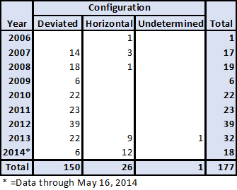
The following chart summarizes data for wells through May 16, 2014 that are not drilled vertically, but that are considered to be conventional, based on depth:
These wells are listed as conventional, but are not drilled vertically.
Note that there have already been more horizontal wells in this group drilled in 2014 than any previous year, showing that the trend is increasing sharply.
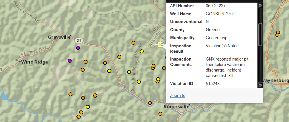
Of the 26 horizontal wells, 12 are considered oil wells, five are gas wells, five are storage wells, three are combination oil and gas, and one is an injection well. These 177 wells have been issued a total of 97 violations, which is a violation per well ratio of 62 percent. 429 permits in have been issued in Pennsylvania to date for non-vertical wells classified as conventional. Greene county has the largest number of horizontal conventional wells, with eight, followed by Bradford (5) and Butler (4) counties.
We can also take a look at this data in a map view:
Conventional, non-vertical wells in Pennsylvania. Please click the expanding arrows icon at the top-right corner to access the legend and other map controls. Please zoom in to access data for each location.
https://www.fractracker.org/a5ej20sjfwe/wp-content/uploads/2014/05/PA_CNV_BlogFeature.png5151004Matt Kelso, BAhttps://www.fractracker.org/a5ej20sjfwe/wp-content/uploads/2025/09/2025-Wordmark-Logo.pngMatt Kelso, BA2014-05-19 16:10:222020-07-21 10:42:26Conventional, Non-Vertical Wells in PA