
The Science Behind OK’s Man-made Earthquakes, Part 2
By Ariel Conn, Seismologist and Science Writer with the Virginia Tech Department of Geosciences
Oklahoma has made news recently because its earthquake story is so dramatic. The state that once averaged one to two magnitude 3 earthquakes per year now averages one to two per day. This same state, which never used to be seismically active, is now more seismically active than California. In terms of understanding the connection between wastewater disposal wells and earthquakes, though, it may be more helpful to look at other states first. Let us explore this issue further in Man-made Earthquakes, Part 2.
How other states handle induced seismicity
In 2010 and 2011, Arkansas experienced a swarm of earthquakes near the town of Greenbrier that culminated in a magnitude 4.7 earthquake. Officials in Arkansas ordered a moratorium on all disposal wells in the area, and earthquake activity quickly subsided.
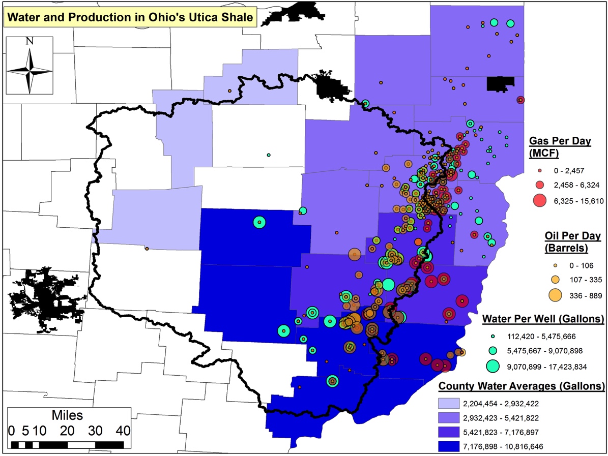
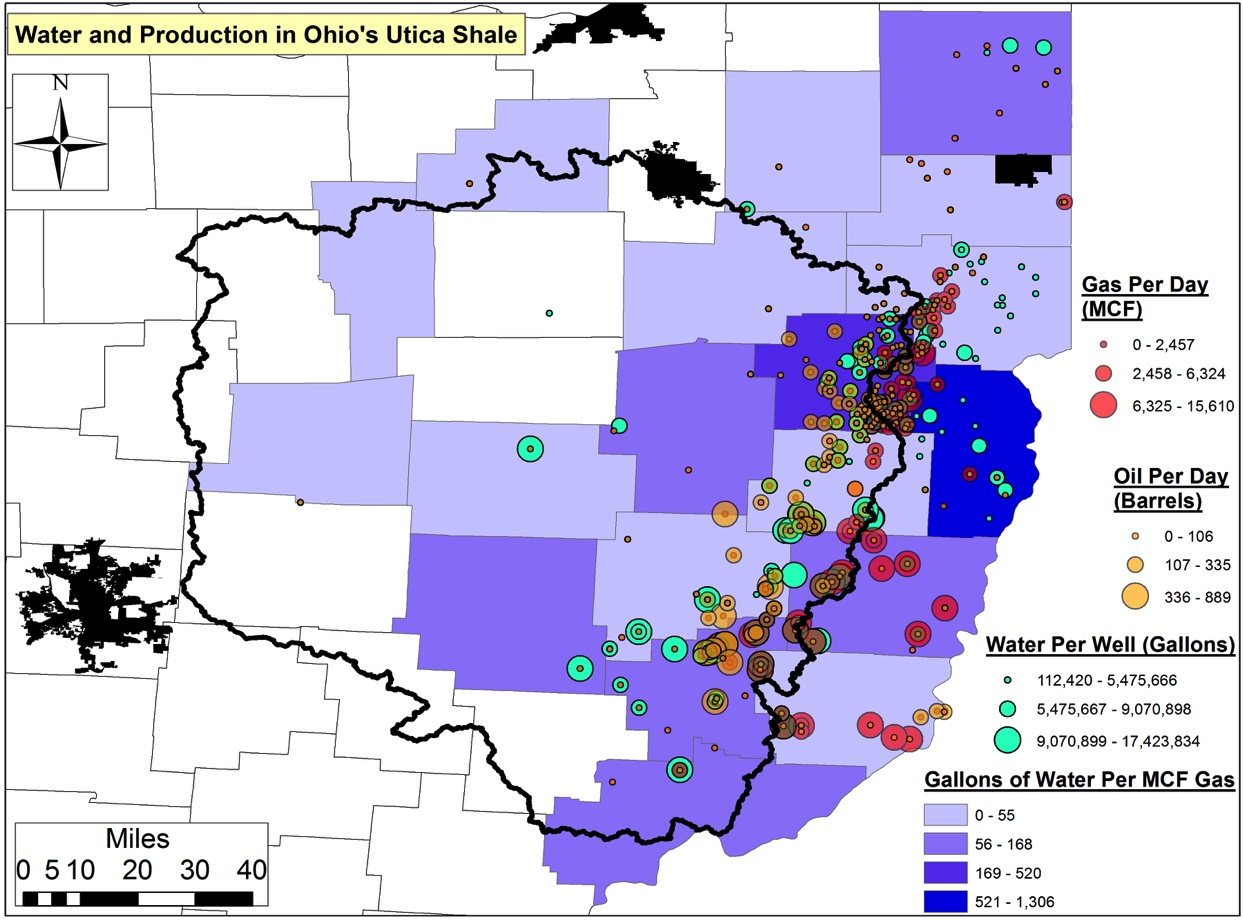
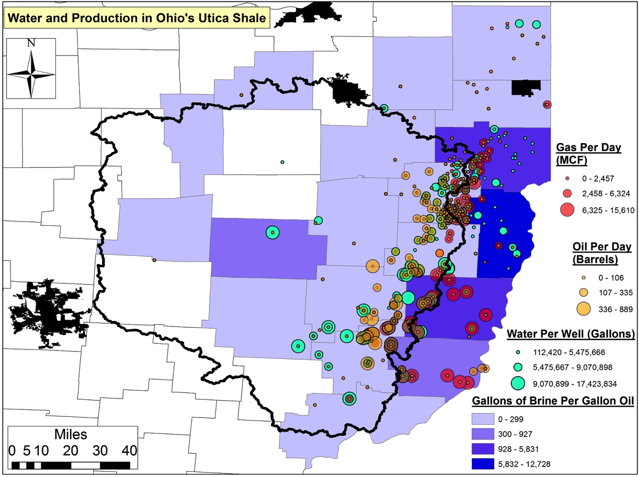
In late 2011, Ohio experienced small earthquakes near a disposal well that culminated in a magnitude 4 earthquake that shook and startled residents. The disposal well was shut down, and the earthquakes subsided. Subsequent research into the earthquake confirmed that the disposal well in question had, in fact, triggered the earthquake. A swarm of earthquakes last year in Ohio shut down another well, and again, after the wastewater injection ceased, the earthquakes subsided.
Similarly in Kansas, after two earthquakes of magnitudes 4.7 and 4.9 shook the state in late 2014, officials ordered wells in two southern counties to decrease the volume of water injected into the ground. Again, earthquake activity quickly subsided.
A seismologist’s toolbox
A favorite saying among scientists is that correlation does not equal causation, and it’s easy to apply that phrase to the correlations seen in Ohio, Arkansas, and Kansas. Yet scientists remain certain that wastewater disposal wells can trigger earthquakes. So what are some of the techniques they use to come to these conclusions? At the Virginia Seismological Observatory (VTSO), two of the tools we used to determine a connection were cross-correlation programs and beach ball diagrams.
Cross-correlation
The VTSO research, which was funded by the National Energy Technology Laboratory, looked specifically at earthquake swarms that have popped up a couple times near a wastewater disposal well in West Virginia. We used a cross-correlation program to distinguish earthquakes that were likely triggered by the nearby well from events that might be natural or related to mining activity.
A seismic station records all of the vibrations that occur around it as squiggly lines. When an earthquake wave passes through, its squiggly lines take on a specific shape, known as a waveform, that seismologists can easily recognize (as an example, the VTSO logo in Fig. 1 was designed using a waveform from one of West Virginia’s potentially induced earthquakes.)
Figure 1. Virginia Tech Seismological Observatory logo w/waveform
For naturally occurring earthquakes, the waveforms will have some variation in shape because they come from different faults in different locations. When an injection well triggers earthquakes, it typically activates faults that are within close proximity, resulting in greater similarities between waveforms. A cross-correlation program is simply a computer program that can run through days, weeks, or months of data from a seismometer to find those similar waveforms. When matching waveforms indicate that earthquake activity is occurring near an injection well – and especially in regions that don’t have a history of seismic activity – we can conclude the earthquakes are triggered by human activity.
Beach Balls
Any earthquake fault, whether it’s active or ancient, is stressed to its breaking point. The difference is that, in places like California that are active, the natural forces against the faults often change, which triggers earthquakes. Ancient faults are still highly stressed, but the ground around them has become more stabilized. However at any point in time, if an unexpected force comes along, it can still trigger an earthquake.

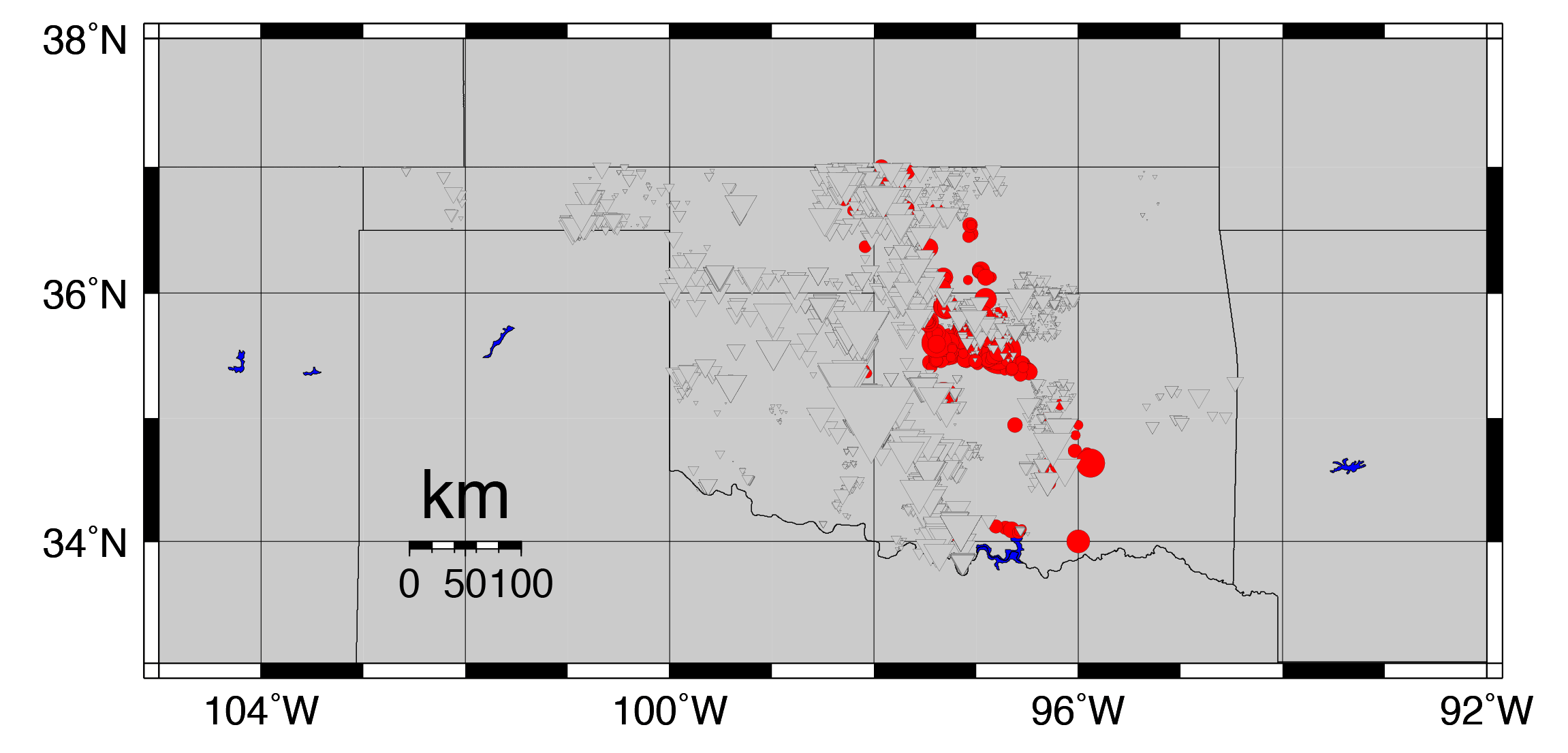
Figure 2. Beach ball diagrams of 16 of the largest earthquakes in Oklahoma in 2014, all showing similar focal mechanisms, which is indicative of induced seismicity.
Earthquake faults don’t all point in the same direction, which means different forces will affect faults differently. Depending on their orientation, some faults might shift in a north-south direction, some might shift in an east-west direction, some might be tilted at an angle, while others are more upright, etc. Seismologists use focal mechanisms to describe the movement of a fault during an earthquake, and these focal mechanisms are depicted by beach ball diagrams (Figure 2). The beach ball diagrams look, literally, like black and white beach balls. Different quadrants of the “beach ball” will be more dominant depending on what type of fault it was and how it moved (See USGS definition of Focal Mechanisms and the “beach ball” symbol).
When an earthquake is triggered by an injection well, it means that the fluid injected into the ground is essentially the straw that broke the camel’s back. Earthquake theory predicts that the forces from an injection well won’t trigger all faults, but only those that are oriented just right. Since we expect that only certain faults with just the right orientation will get triggered, that means we also expect the earthquakes to have similar focal mechanisms, and thus, similar beach ball diagrams. And that’s exactly what we see in Oklahoma.
Cross-correlation programs and beach ball diagrams are only two tools we used at the VTSO to confirm which earthquakes were induced, but seismologists have many means of determining if an earthquake is induced or natural.
Limitations of science?
With so much strong scientific evidence, why can people in industry still claim there isn’t enough science to officially confirm that an injection well triggered an earthquake? In some cases, these claims are simply wrong. In other cases, though, especially in Oklahoma, the problem is that no one was monitoring the disposal wells and the earthquakes from the start. Well operators were not required to publicly track the volumes of water they injected into wells until recently, and no one monitored for nearby earthquake activity. The big problem is not a lack of scientific evidence, but a lack of data from industry to perform sufficient research. Scientists need information about the history, volume, and pressure of fluid injection at a disposal well if they’re to confirm whether or not earthquakes are triggered by it. Often, that information is proprietary and not publically available, or it may not exist at all.
At this point though, two other factors make direct correlations between injection wells and earthquakes in Oklahoma even more difficult:
- So many wells have injected signficiant volumes of water in close enough proximity that pointing a finger at a specific well is more challenging.
- A large number of wells have injected water for so many years, that the earthquakes are migrating farther and farther from their original source. Again, pointing a finger at a specific well gets harder with time.
What we know
We know what induced seismicity is and why it occurs. We know that if a wastewater injection well disposes of large volumes of fluids deep underground in a region that has existing faults, it will likely trigger earthquakes. We know that if a region previously had few earthquakes, and then sees an uptick in earthquakes after wastewater injection begins, the earthquakes are likely induced. We know that if we want to understand the situation better, we need more seismic stations near disposal wells so we can more accurately monitor the area for seismicity both before and after the well becomes active.
What don’t we know?
We don’t know how big an induced earthquake can get. Oklahoma’s largest earthquake, which was also the largest induced earthquake ever recorded in the United States, was a magnitude 5.6. That’s big enough to cause millions of dollars of damage. Worldwide, the largest earthquake suspected to be induced occurred near the Koyna Dam in India, where a magnitude 6.3 earthquake killed nearly 200 people in 1967.
Can an earthquake that large occur in the central U.S.? The best guess right now: yes.
Seismologists suspect that an induced earthquake could get as big as the size of the fault. If a fault is big enough to trigger a magnitude 7 or 8 earthquake, then that is potentially how large an induced earthquake could be. In the early 1800s, three earthquakes between magnitudes 7 and 8 struck along the New Madrid Fault Zone near St. Louis, Missouri. Toward the end of the 1800s, a magnitude 7 earthquake shook Charleston, South Carolina. In those two areas, injection wells could potentially trigger very large earthquakes.
We have no historic record of earthquakes that large in Oklahoma, so right now, the best guess is that the largest an earthquake could get there would be between a magnitude 6 and 6.5. That would be big enough to cause significant damage, injuries, and possibly death.
The solution
What’s the take-home message from all of this?
- First, the science exists to back up the conclusion that wastewater injection wells trigger earthquakes.
- Second, if we want to get a better feel for which wells are more problematic, we need funding, seismic stations, and staff to monitor seismic activity around all high-volume injection wells, along with a history of injection times, volumes and pressures at the well.
- Third, this is a problem that, if left unchecked, has the potential to result in major damage, incredible expense, and possibly loss of life.
Induced earthquakes are a real phenomenon. While more research is necessary to help us better understand the intricacies of these events and to identify correlations in complex cases, the general cause of the earthquake swarms in Oklahoma and other states is not a mystery. They are man-made problems, backed up by decades of scientific research. They have the potential to create significant damage, but we have the wherewithal to prevent them. We don’t need to go to the extreme of shutting down all wells, but rather, we just need to be able to monitor the wells and ensure that they don’t trigger earthquakes. If a well does trigger an earthquake, then at that point, the well operators can either experiment with significantly decreasing the volume of water that’s injected, or the well can be shut down completely. Understanding and acknowledging the connection between injection wells and earthquakes will make induced seismicity a much easier problem to solve.


