Ethanol and fracking

North American Ethanol’s Land, Water, Nutrient, and Waste Impact

Corn Ethanol and Fracking – Similarities Abound

Even though it is a biofuel and not a fossil fuel, in this post we discuss the ways in which the corn ethanol production industry is similar to the fracking industry. For those who may not be familiar, biofuel refers to a category of fuels derived directly from living matter. These may include:

  1. Direct combustion of woody biomass and crop residues, which we recently mapped and outlined,
  2. Ethanol1 produced directly from the fermentation of sugarcanes or indirectly by way of the intermediate step of producing sugars from corn or switchgrass cellulose,
  3. Biodiesel from oil crops such as soybeans, oil palm, jatropha, and canola or cooking oil waste,2 and
  4. Anaerobic methane digestion of natural gas from manures or human waste.

Speaking about biofuels in 2006, J. Hill et al. said:

To be a viable substitute for a fossil fuel, an alternative fuel should not only have superior environmental benefits over the fossil fuel it displaces, be economically competitive with it, and be producible in sufficient quantities to make a meaningful impact on energy demands, but it should also provide a net energy gain over the energy sources used to produce it.

Out of all available biofuels it is ethanol that accounts for a lion’s share of North American biofuel production (See US Renewables Map Below). This trend is largely because most Americans put the E-10 blends in their tanks (10% ethanol).3 Additionally, the Energy Independence and Security Act of 2007 calls for ethanol production to reach 36 billion gallons by 2022, which would essentially double the current capacity (17.9 billion gallons) and require the equivalent of an additional 260 refineries to come online by then (Table 1, bottom).

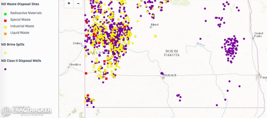
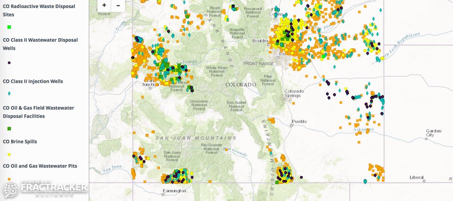
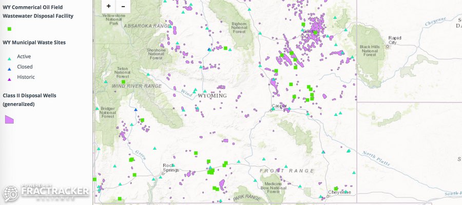
US Facilities Generating Energy from Biomass and Waste along with Ethanol Refineries and Wind Farms


View map fullscreen | How FracTracker maps work

But more to the point… the language, tax regimes, and potential costs of both ethanol production and fracking are remarkably similar. (As evidenced by the quotes scattered throughout this piece.) Interestingly, some of the similarities are due to the fact that “Big Ag” and “Big Oil” are coupled, growing more so every year:

The shale revolution has resulted in declining natural gas and oil prices, which benefit farms with the greatest diesel, gasoline, and natural gas shares of total expenses, such as rice, cotton, and wheat farms. However, domestic fertilizer prices have not substantially fallen despite the large decrease in the U.S. natural gas price (natural gas accounts for about 75-85 percent of fertilizer production costs). This is due to the relatively high cost of shipping natural gas, which has resulted in regionalized natural gas markets, as compared with the more globalized fertilizer market. (USDA, 2016)

Ethanol’s Recent History

For background, below is a timeline of important events and publications related to ethanol regulation in the U.S. in the last four decades: 

Benefits of Biofuels

[Bill] Clinton justified the ethanol mandate by declaring that it would provide “thousands of new jobs for the future” and that “this policy is good for our environment, our public health, and our nation’s farmers—and that’s good for America.” EPA administrator Carol Browner claimed that “it is important to our efforts to diversify energy resources and promote energy independence.” – James Bovard citing Peter Stone’s “The Big Harvest,” National Journal, July 30, 1994.

Of the 270 ethanol refineries we had sufficient data for, we estimate these facilities employ 235,624 people or 873 per facility and payout roughly $6.18-6.80 billion in wages each year, at an average of $22.9-25.2 million per refinery. These employees spend roughly 423,000 hours at the plant or at associated operations earning between $14.63 and $16.10 per hour including benefits. Those figures amount to 74-83% of the average US income. In all fairness, these wages are 13-26% times higher than the farming, fishing, and forestry sectors in states like Minnesota, Nebraska, and Iowa, which alone account for 33% of US ethanol refining.

Additional benefits of ethanol refineries include the nearly 179 million tons of CO2 left in the field as stover each year, which amounts to 654,532 tons per refinery. Put another way – these amounts are equivalent to the annual emissions of 10.7 million and 39,194 Americans, respectively.

Finally, what would a discussion of ethanol refineries be without an estimate of how much gasoline is produced? It turns out that the 280 refineries (for which we have accurate estimates of capacity) produce an average of 71.93 million gallons per year and 20.1 billion gallons in total. That figure represents 14.3% of US gasoline demand.

Costs of Biofuels

Direct Costs

Biofuel expansions such as those listed in the timeline above and those eluded to by the likes of the IPCC have several issues associated with them. One of which is what Pimentel et al. considered an insufficient – and to those of us in the fracking NGO community, familiar sounding – “breadth of relevant expertise and perspectives… to pronounce fairly and roundely on this many-sided issue.”

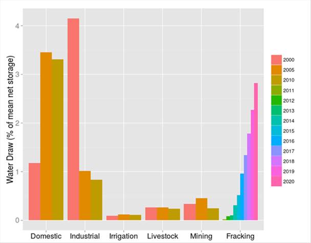
The above acts and reports in the timeline prompted many American farmers to double down on corn at the expense of soybeans, which caused Indirect Land Use Change (ILUC); the global soy market skyrocketed. This, in turn, prompted the clearing and/or burning of large swaths of the Amazonian rainforests and tropical savannas in Brazil, the world’s second-leading soy producer. More recently, large swaths of Indonesia and Malaysia’s equally biodiverse peatland forests have been replaced by palm oil plantations (Table 2 and Figure 3, bottom). In the latter countries, forest displacement is increasing by 2.7-5.3% per year, which is roughly equal to the the rate of land-use change associated with hydraulic fracturing here in the US4 (Figure 1).


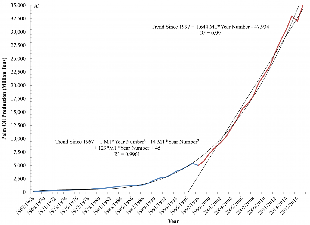
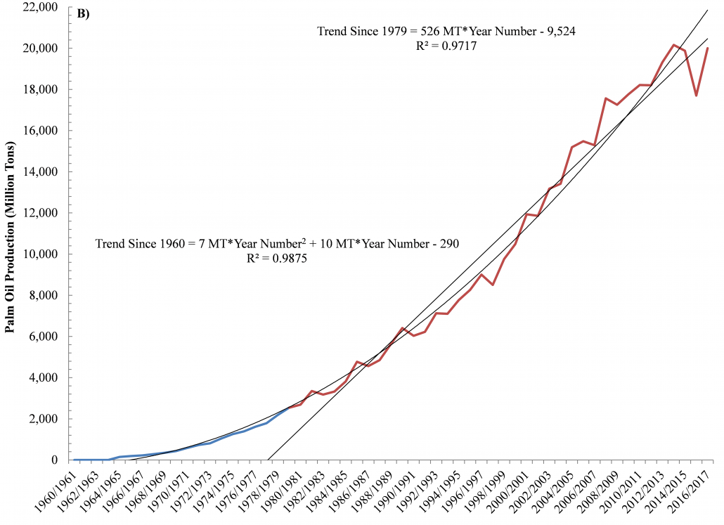
Figures 1A and 1B. Palm Oil Production in A) Indonesia and B) Malaysia between 1960 and 2016.

There is an increasing amount of connectivity between disparate regions of the world with respect to energy consumption, extraction, and generation. These connections also affect how we define renewable or sustainable:

In a globalized world, the impacts of local decisions about crop preferences can have far reaching implications. As illustrated by an apparent “corn connection” to Amazonian deforestation, the environmental benefits of corn-based biofuel might be considerably reduced when its full and indirect costs are considered. (Science, 2007)

These authors pointed to the fact that biofuel expectations and/or mandates fail to account for costs associated with atmospheric – and leaching – emissions of carbon, nitrogen, phophorus, etc. during the conversion of lands, including diverse rainforests, peatlands, savannas, and grasslands, to monocultures. Also overlooked were:

  • The ethical concerns associated with growing malnourishment from India to the United States,
  • The fact that 10-60%5 more fossil fuel derived energy is required to produce a unit of corn ethanol than is actually contained within this very biofuel, and
  • The tremendous “Global land and water grabbing” occuring in the name of natural resource security, commodification, and biofuel generation.

Sacrificing long-term ecological/food security in the name of short-term energy security has caused individuals and governments to focus on taking land out of food production and putting it into biofuels.

The rationale for ethanol subsidies has continually changed to meet shifting political winds. In the late 1970s ethanol was championed as a way to achieve energy independence. In the early 1980s ethanol was portrayed as salvation for struggling corn farmers. From the mid and late 1980s onward, ethanol has been justified as saving the environment. However, none of those claims can withstand serious examination. (James Bovard, 1995)

This is instead of going the more environmentally friendly route of growing biofuel feedstocks on degraded or abandoned lands. An example of such an endeavor is the voluntary US Conservation Reserve Program (CRP), which has stabilized at roughly 45-57 thousand square miles of enrolled land since 1990, even though the average payout per acre has continued to climb (Figure 2).

The Average Subsidy to Farmers Per Acre of Conservation Reserve Program (CRP) between 1986 and 2015.

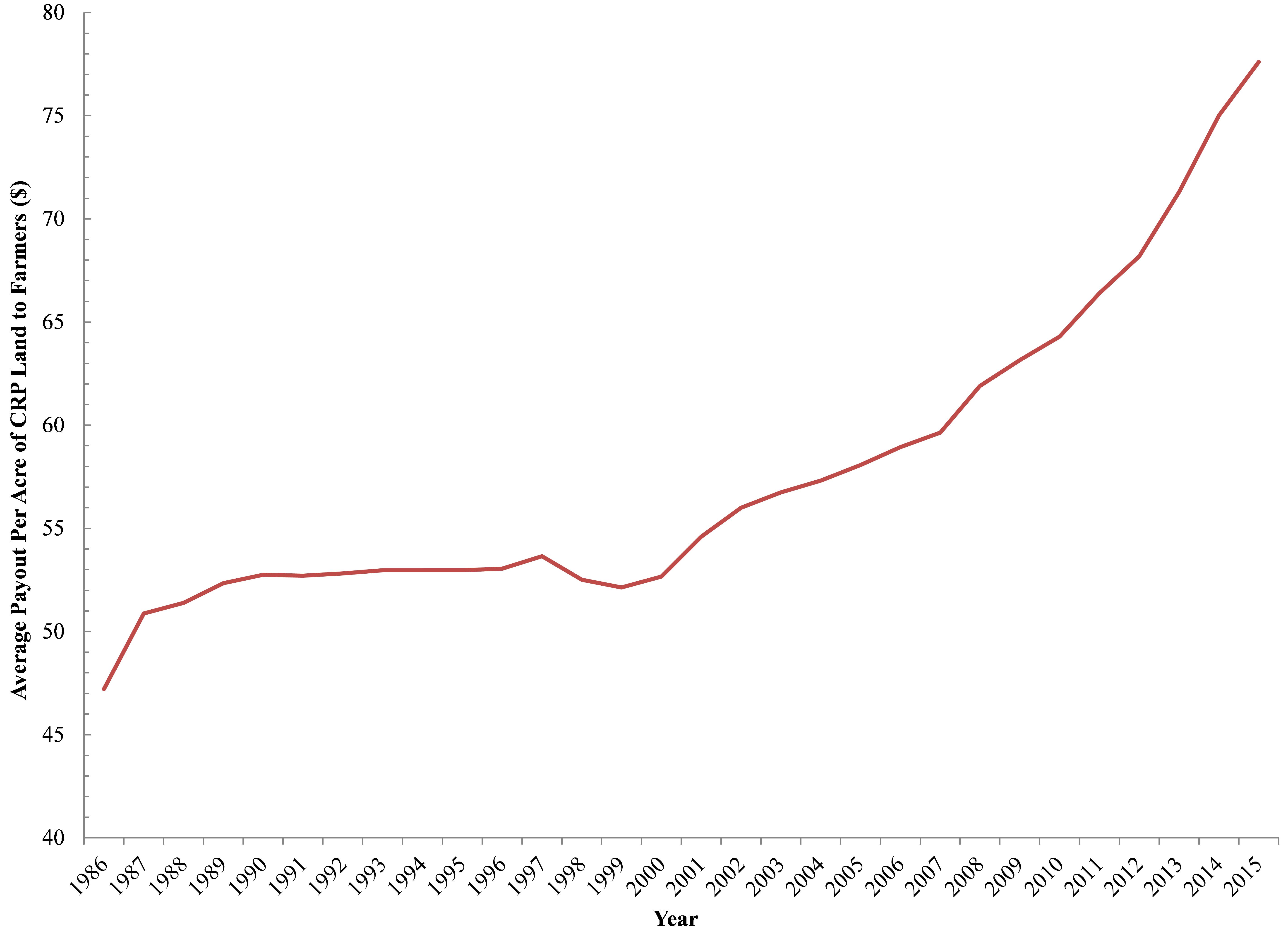
Figure 2. The Average Subsidy to Farmers Per Acre of Conservation Reserve Program (CRP) between 1986 and 2015.

The primary goals of the CRP program are to provide an acceptable “floor” for commodity prices, reduce soil erosion, enhance wildlife habitat, ecosystem services, biodiversity, and improve water quality on highly erodible, degraded, or flood proned croplands. Interestingly CRP acreage has declined by 27% since a high of 56 thousand square miles prior to the Energy Independence and Security Act of 2007 being passed. Researchers have pointed to the fact that corn ethanol production on CRP lands would create a carbon debt that would take 48 years to repay vs. a 93 year payback period for ethanol on Central US Grasslands.

To quote Fred Magdoff in The Political Economy and Ecology of Biofuels:

Alternative fuel sources are attractive because they can be developed and used without questioning the very workings of the economic system — just substitute a more “sustainable,” “ecologically sound,” and “renewable” energy for the more polluting, expensive, and finite amounts of oil. People are hoping for magic bullets to “solve” the problem so that capitalist societies can continue along their wasteful growth and consumption patterns with the least disruption. Although prices of fuels may come down somewhat — with dips in the business cycle, higher rates of production, or a burst in the speculative bubble in the futures market for oil — they will most likely remain at historically high levels as the reserves of easily recovered fuel relative to annual usage continues to decline.

Indirect Costs: Ethanol, Fertilizers, and the Gulf of Mexico Dead Zone

This is the Midwest vs. the Middle East. It’s corn farmers vs. the oil companies. – Dwaney Andreas in Big Stink on the Farm by David Greising

Sixty-nine percent6 of North America’s ethanol refineries are within the Mississippi River Basin (MRB). These refineries collectively rely on corn that receives 1.9-5.1 million tons of nitrogen each year, with a current value of $1.06-2.91 billion dollars or 9,570-26,161 tons of nitrogen per refinery per year (i.e. $5.42-14.81 million per refinery per year). These figures account for 27-73% of all nitrogen fertilizer used in the MRB each year. More importantly, the corn acreage receiving this nitrogen leaches roughly 0.81-657 thousand tons of it directly into the MRB. Such a process amounts to 5-44% of all nitrogen discharged into the Gulf of Mexico each year and 1.7-13.8 million tons of algae responsible for the Gulf’s growing Dead Zone.

Midwest/Great Plains US Ethanol Refineries and Crop Residue Production

Leaching of this nitrogen is analogous to flushing $45.7-371.6 million dollars worth of precious capital down the drain. Put another way, these dollar figures translate into anywhere between 55% and an astonishing 4.53 times Direct Costs to the Gulf’s seafood and tourism industries of the Dead Zone itself.

These same refineries rely on corn acreage that also receives 0.53-2.61 million tons of phosphorus each year with a current value of 0.34-1.66 billion dollars. Each refinery has a phosphrous footprint in the range of 2,700 to 13,334 tons per year (i.e., $1.72-8.47 million). We estimate that 25,399-185,201 tons of this fertilizer phosphorus is leached into the the MRB, which is equivalent to 19% or as much as 1.42 times all the phosphorous dischared into the Gulf of Mexico per year. Such a process means $16.13-117.60 million is lost per year.

Together, the nitrogen and phosphorus leached from acreage allocated to corn ethanol have a current value that is between 75% and nearly 6 times the value lost every year to the Gulf’s seafood and tourism industries.

Indirect Costs: Fertilizer and Herbicide Costs and Leaching

The 270 ethanol refineries we have quality production data for are relying on corn that receives 367,772 tons of herbicide and insecticide each year, with a current value of $6.67 billion dollars or 1,362 tons of chemical preventitive per refinery per year (i.e. $24.7 million per refinery per year). More importantly the corn acreage receiving these inputs leaches roughly 15.8-128.7 thousand tons of it directly into surrounding watersheds and underlying aquifers. Leaching of these inputs is analogous to flushing $287 million to $2.3 billion dollars down the drain.

What’s Next?

During the recent Trump administration EPA, USDA, DOE administrator hearings, the Renewable Fuel Standard (RFS) was cited as critical to American energy independence by a bipartisan group of 23 senators. Among these were Democratic senator Amy Klobuchar and Republican Chuck Grassley, who co-wrote a letter to new EPA administrator Scott Pruitt demanding that the RFS remains robust and expands when possible. In the words of Democratic Senator Heidi Heitkamp – and long-time ethanol supporter – straight from the heart of the Bakken Shale Revolution in North Dakota:

The RFS has worked well for North Dakota farmers, and I’m fighting to defend it. As we’re doing today in this letter, I’ll keep pushing in the U.S. Senate for the robust RFS [and Renewable Volume Obligations (RVOs)] we need to support a thriving biofuels industry and stand up for biofuels workers. Biofuels create good-paying jobs in North Dakota and help support our state’s farmers, who rely on this important market – particularly when commodity prices are challenging.

Furthermore, the entire Iowa congressional delegation including the aforementioned Sen. Grassley joined newly minted USDA Secretary Sonny Perdue when he told the Iowa Renewable Fuels Association:

You have nothing to worry about. Did you hear what he said during the campaign? Renewable energy, ethanol, is here to stay, and we’re going to work for new technologies to be more efficient.

How this advocacy will play out and how the ethanol industry will respond (i.e., increase productivity per refinery or expand the number of refineries) is anybody’s guess. However, it sounds like the same language, lobbying, and advertising will continue to be used by the Ethanol and Unconventional Oil and Gas industries. Additional parallels are sure to follow with specific respect to water, waste, and land-use.

Furthermore, as both industries continue their ramp up in research and development, we can expect to see productivity per laborer to continue on an exponential path. The response in DC – and statehouses across the upper Midwest and Great Plains – will likely be further deregulation, as well.

From a societal perspective, an increase in ethanol production/grain diversion away from people’s plates has lead to a chicken-and-egg positive feedback loop, whereby our farmers continue to increase total and per-acre corn production with less and less people. In rural areas, mining and agriculture have been the primary employment sectors. A further mechanization of both will likely amplify issues related to education, drug dependence, and flight to urban centers (Figures 4A and B).

We still don’t know exactly how efficient ethanol refineries are relative to Greenhouse Gas Emissions per barrel of oil. By merging the above data with facility-level CO2 emissions from the EPA Facility Level Information on Greenhouse gases Tool (FLIGHT) database we were able to match nearly 200 of the US ethanol refineries with their respective GHG emissions levels back to 2010. These facilities emit roughly:

  • 195,116 tons of CO2 per year, per facility,
  • A total of 36.97 million tons per year (i.e., 2.11 million Americans worth of emissions), and
  • 22,265 tons of CO2 per barrel of ethanol produced.

Emissions from ethanol will increase to 74.35 million tons in 2022 if the Energy Independence and Security Act of 2007’s prescriptions run their course. Such an upward trend would be equivalent to the GHG emissions of somewhere between that of Seattle and Detroit.

What was once a singles match between Frackers and Sheikhs may turn into an Australian Doubles match with the Ethanol Lobby and Farm Bureau joining the fray. This ‘game’ will only further stress the food, energy, and water (FEW) nexus from California to the Great Lakes and northern Appalachia.

We are on a thinner margin of food security, just as we are on a thinner margin of oil security… The [World] Bank implicitly questions whether it is wise to divert half of the world’s increased output of maize and wheat over the next decade into biofuels to meet government “mandates.” – Ambrose Evans-Pritchard in The Telegraph

Will long-term agricultural security be sacrificed in the name of short-term energy independence?

US and Global Corn Production and Acreage between 1866 and 2015.

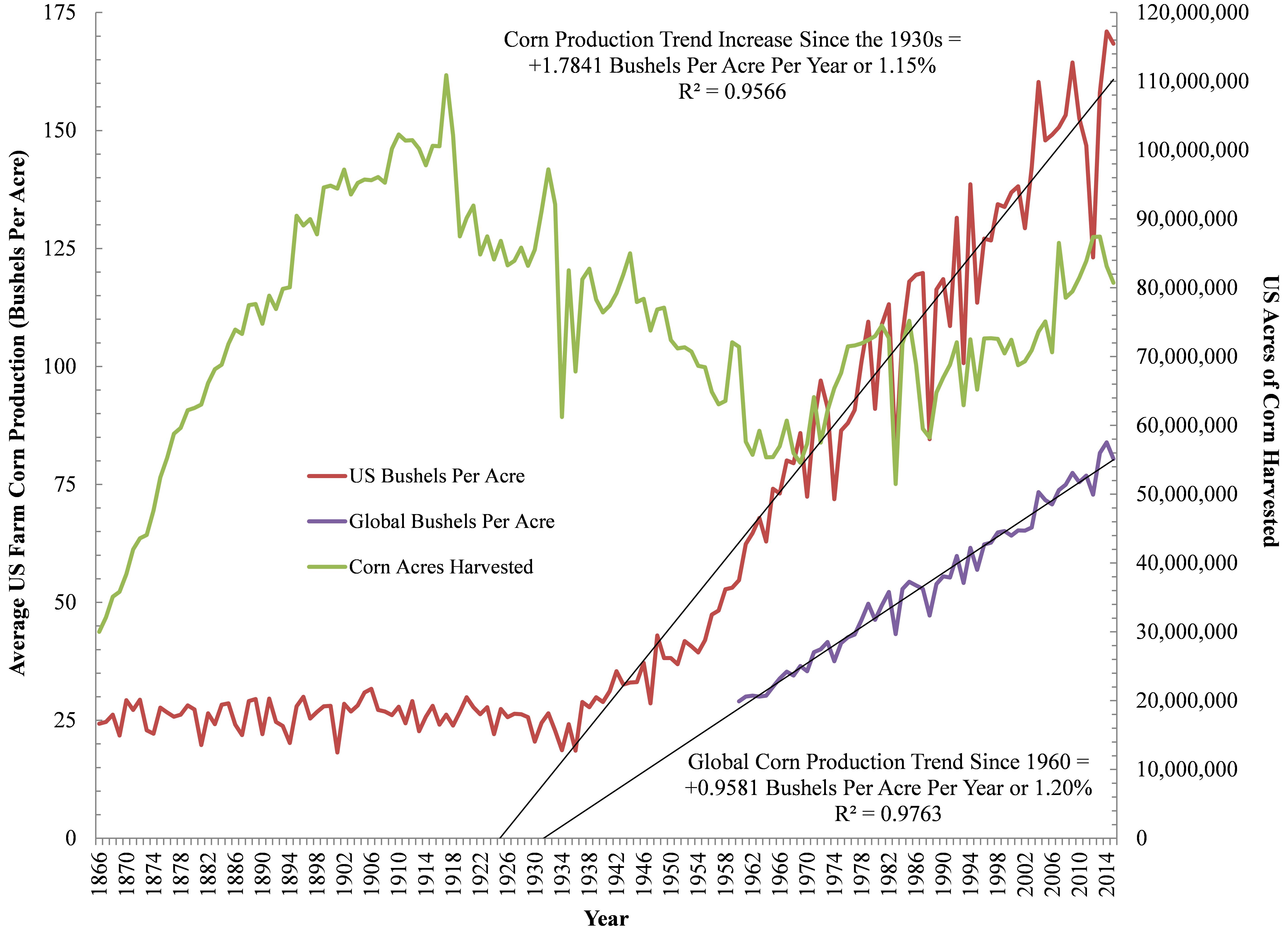
Figure 3. US and Global Corn Production and Acreage between 1866 and 2015.

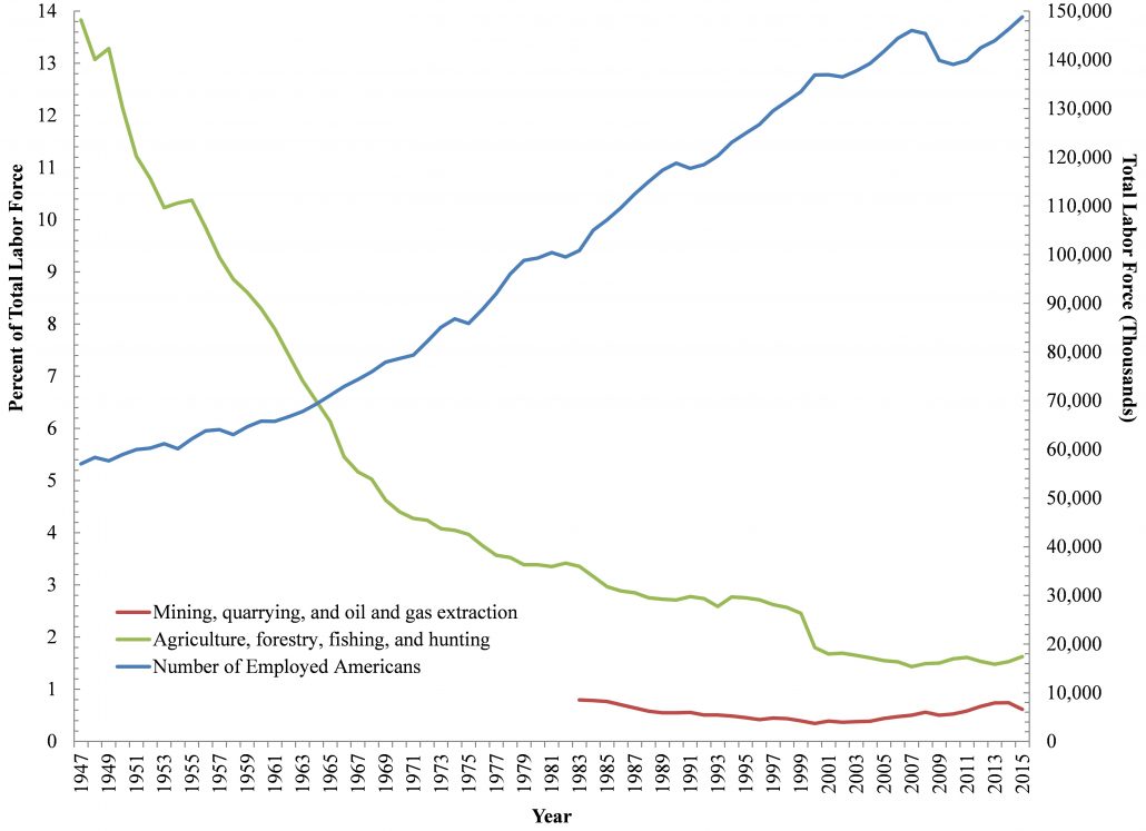
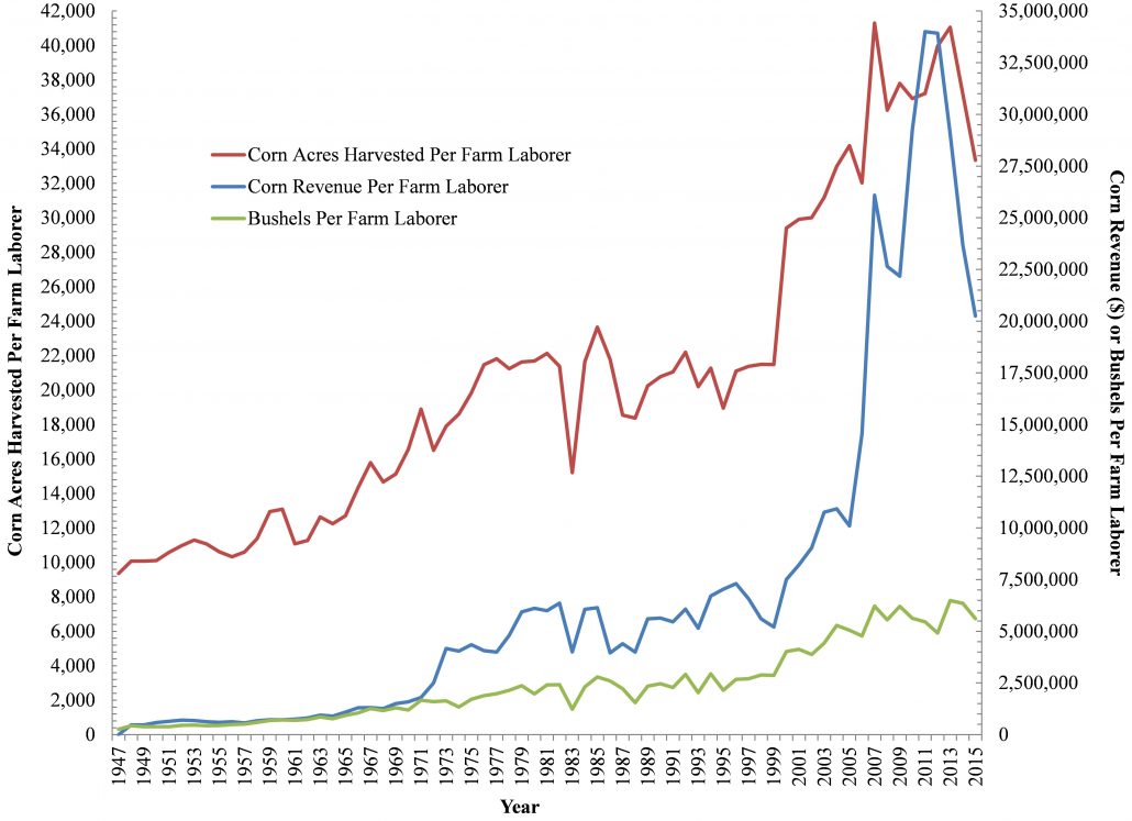
Figures 4A and 4B. A) Number of Laborers in the US Mining, Oil and Gas, Agriculture, Forestry, Fishing, and Hunting sector and B) US Corn Production Metrics Per Farm Laborer between 1947 and 2015.

Ethanol Tables

Table 1. Summary of our Corn Ethanol Production, Land-Use, and Water Demand analysis

Gallons of Corn Ethanol Produced Per Year 17,847,616,000
Bushels of Corn Needed 6,374,148,571
Percent of US Production 44.73%
Land Needed 104,372,023 acres
“” 163,081 square miles
Percent of Contiguous US Land 5.51%
Percent of US Agricultural Land 11.28%
Gallons of Water Needed 49.76 trillion (i.e. 3.55 million swimming pools)
Gallons of Water Per Gallon of Oil 2,788
Average and Total Site/Industry Capacity
Average Corn Ethanol Production Per Existing or Under Construction Facility (n = 257) 69,717,250
Gallons of Corn Ethanol Produced Per Year 17,847,616,000
Difference Between 2022 Energy Independence and Security Act of 2007 36 Billion Gallon Mandate 18,152,384,000
# of New Refineries Necessary to Get to 2022 Levels 260
Percent Increase Over Current Facility Inventory 1.7
IEA 2009 World Energy Outlook 250-620% Increase Predictions for 2030
250% 44,619,040,000
# of New Refineries Necessary 640
Percent Increase Over Current Facility Inventory 150.00
620% 110,655,219,200
# of New Refineries Necessary 1,587
Percent Increase Over Current Facility Inventory 520.00

Table 2. Global Population Growth and Corn and Soybean Productivity Trends.

Percent Change Metric
+1.13% Global Population Growth Trend
Corn (Bushels Per Acre)
+1.15% Per Year United States
+1.20% Per Year Global
Soybean (Tons Per Acre)
+0.9% Per Year United States
+1.5% Per Year Brazil
Palm Oil (Tons)
+5.1% Per Year Indonesia
+2.7% Per Year Malaysia

References and Footnotes

  1. Ethanol as defined in the Ohio Revised Code (ORC) Corporation Franchise Tax 5733.46 means “fermentation ethyl alcohol derived from agricultural products, including potatoes, cereal, grains, cheese whey, and sugar beets; forest products; or other renewable resources, including residue and waste generated from the production, processing, and marketing of agricultural products, forest products, and other renewable resources that meet all of the specifications in the American society for testing and materials (ASTM) specification D 4806-88 and is denatured as specified in Parts 20 and 21 of Title 27 of the Code of Federal Regulations.”
  2. A) Pyrolysis is included in the biofuel category and involves the anaerobic decay of cellulose rich feedstocks such as switchgrass at high temperatures producing synthetic diesel or syngas, and
    B) According to many researchers biofuels made from waste biomass or crops grown on degraded and abandoned lands with warm-season prairie grasses and legumes incur little or no carbon debt and provide “immediate and sustained Greenhouse Gas (GHG) advantages” by rehabilitating soil health and capturing, rather than emitting by way of increased fertilizer use, various forms of nitrogen including N2O, NO3, and NO2.
  3. According to Fred Magdoff, the ethanol complex is lobbying for “more automobile engines capable of using E-85 (85 percent ethanol, 15 percent gasoline) for which there are currently 2,710 fueling stations across the country although 56% of them are in just nine states: 1) Wisconsin (117), 2) Missouri (107), 3) Minnesota (335), 4) Michigan (174), 5) Indiana (172), 6) Illinois (221),  7) Iowa (193), 8) Texas (99), and 9) Ohio (97). Some states are mandating a mixture greater than 10 percent. Ethanol can’t be shipped together with gasoline in pipelines because it separates from the mixture when moisture is present, so it must be trucked to where it will be mixed with gasoline.” The E-85 blend comes with its own costs including higher emissions of CO, VOC, PM10, SOx, and NOx than gasoline.
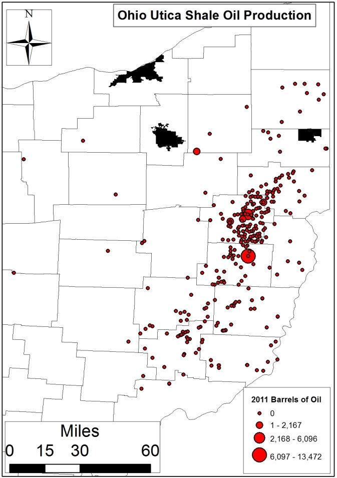
  4. McClaugherty, C., Auch, W. Genshock, E. and H. Buzulencia. (2017). Landscape impacts of infrastructure associated with Utica shale oil and gas extraction in eastern Ohio, Ecological Society of America, 100th Annual Meeting, Baltimore, MD, August, 2015.
  5. Hill et al. recently indicated “Ethanol yields 25% more energy than the energy invested in its production, whereas biodiesel yields 93% more.”
  6. An additional 9-10 refineries or 73% of all ethanol refineries are within 25 miles of the Mississippi River Basin.

By Ted Auch, PhD, Great Lakes Program Coordinator, FracTracker Alliance

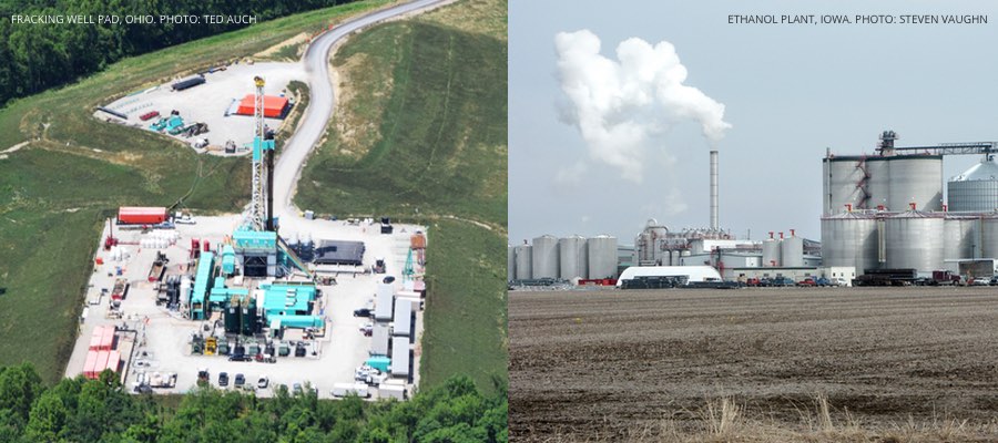
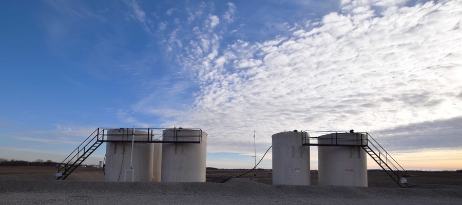
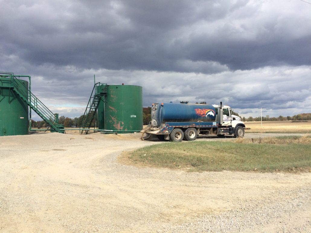
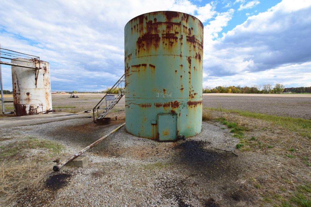
Cover photo, left: Oil and gas well pad, Ohio. Photo by Ted Auch.
Cover photo, right: A typical ethanol plant in West Burlington, Iowa. Photo by Steven Vaughn.


Data Downloads

Click on the links below to download the datasets used to create the maps in this article.

  1. Detailed US Ethanol water, land, chemical fertilizer, and herbicide demand
  2. Estimates of North American Ethanol Refinery’s water and land-use demand

Radium Watersheds a Risk

By Greg Pace – Columbus Community Bill of Rights, and Julie Weatherington-Rice – Environmental Consultant

columbus_classiimap

Figure 1. Map of Columbus, OH Watersheds and Class II Injection Wells

Most Ohio residents are unaware of the frack fluid deep underground injection occurring north of Columbus, underneath the region’s source water protection watersheds (Figure 1).

Materials injected are liquids that have as much as ten times the salt concentration of sea-water. Mixed with this “brine” solution is a combination from hundreds of chemicals that are used in different stages of horizontal hydraulic fracturing, the process used to extract natural gas, petroleum, and hydrocarbon liquids used to make industrial materials such as plastics. BTEX compounds including benzene are always present in the wastewater, along with formaldehyde, bromides, ethylene glycol (antifreeze), and arsenic, with many other carcinogenic and otherwise highly-toxic substances.

Radioactivity of Shale Gas Wastewater

One of the biggest questions in this mix of toxic disposal is how much radioactive content exists. Radium-226 is most worrisome, as it has a very long half-life (1,600 years). It is water-soluble and, once it enters the human body, seeks to find a home in our bones where it will emit its cell-formation-destabilizing effects for the remainder of our lifetime. This radionuclide is known to cause leukemia, bone cancers, blood disorders, and other diseases.

The state of Ohio does not monitor the content of materials that are injected into our Class II injection wells deep in the ground. This oil and gas waste can come from anywhere, including Pennsylvania’s Marcellus shale, which is the most highly-radioactive geology of all the shale plays in the country. Radium-226 readings as high as 15,000 pico-curies per liter have been read in Marcellus shale brines. The EPA drinking water limit for radium-226 is 5 pico-curies per liter, which puts the Marcellus reading at 3,000 times higher than the drinking water limit.

Exposure through drinking water is a pathway to human disease from radium-226. Once oil and gas waste is disposed of underground in a sandstone or limestone layer, the fluids are subject to down-gradient movement, wicking through capillary action, and seepage over time. This means that the highly radioactive wastewater could eventually end up in our underground drinking water sources, creating radium watersheds. This practice is putting our watersheds at risk from radioactive contamination for hundreds of years, at least.

Can injected fluids migrate?

Depending on whether you confer with a geologist who works with the oil and gas industry, or from an independent geologist, you will get a different opinion on the likelihood of such a pollution event occurring. Industry geologists mostly claim that deep injection leaves very low risk of water contamination because it will not migrate from the planned area of injection. On the other hand, independent geologists will tell you that it is not a matter of if the liquids will migrate, but how and when. The ability to confirm the geology of the underground area layer of injection “storage” is not exact, therefore accuracy in determining the probability for migration over time is poor.

Figure 2. Ohio Utica Brine Production and Class II Injection Well Disposal


View Map Fullscreen | How FracTracker maps work

We do know, however, that all underground systems in Ohio leak – Research by The Ohio State University and the US Geological Survey show that the age of the water in brine formations is far younger than the age of the rock deposits they are found in. See where wastewater is being created and disposed of in Ohio using the dynamic map above (Figure 2).

Spill Risks to Columbus, OH Water

According to area geologist, Dr. Julie Weatherington-Rice, the source for Columbus’s water to the north is mostly from surface water. This water comes from the Delaware and Morrow county watersheds that feed into sources such as the Hoover and Alum Creek reservoirs. The major threat from injection wells to our watershed is from spills, either from trucks or from storage at the injection well sites themselves.

Dead fish floating in Vienna area pond contaminated by injection well system spill Source: MetropolitanEnegineering Consulting & Forensics-Expert Engineers

Figure 3. Dead fish floating in Vienna area pond contaminated by injection well system spill. Source: MetropolitanEnegineering Consulting & Forensics-Expert Engineers

In April 2015, as much as 8,000 gallons of liquid leaked from a malfunctioning pipe in the storage apparatus of an oil/gas waste storage and injection well site in Vienna, OH. This caused a wildlife kill in two ponds (Figure 3), and the spill was not contained until 2/3 mile downstream in a tributary. The firm who owned the facility was found negligent in that they did not install a required containment liner for spills. The incident was discovered by neighboring residents, but apparently employees knew of the leak weeks before. Of note in this incident was that Ohio Department of Natural Resources, the regulatory agency that oversees all oil/gas production activity in Ohio including injection, stated that there was “minimal impact to wildlife.”

Brine tanker rollover near Barnesville, OH spilled 5,000 gal. of produced brine. Source: Barnesville, OH Fire Department

Figure 4. Brine tanker rollover near Barnesville, OH spilled 5,000 gal. of produced brine. Source: Barnesville, OH Fire Department

In March, 2016, a tanker truck carrying produced waste from a hydraulically fractured well pad overturned outside of the Village of Barnesville, Ohio (Figure 4). The truck spilled 5,000 gallons of liquid waste into a field that led into a tributary, leading the fluids to enter one of the city’s three drinking water supply reservoirs. The water source was shut down for more than two months while regulators determined if water levels were safe for consumption. There was a noted spike in radium-226 levels during water testing immediately after the spill.

Of greatest concern is that, although many millions of gallons of frack waste have been injected into the wells north of Columbus over the past few years, we expect that this activity will increase. For the first time, the United States began exporting its own natural gas in 2016, to regions such as Europe and South America. As the industry consolidates from the depression of oil prices over the past two years and begins to ramp up again, we expect the extraction activity in the Marcellus and especially Utica to increase to levels beyond what we have seen since 2011. The levels of injection will inevitably follow, so that injection wells in Ohio will receive much more than in the past. The probability of spills, underground migration, and human-induced earthquakes may increase steeply, as well.

An Aging Disposal Infrastructure

On our Columbus Community Bill of Rights website, we show pictures of some of the Class II injection wells in Morrow County, most of them converted from legacy production wells. These old wells are located in played out oil/gas fields that may still be producing or have abandoned but not plugged (closed) wells, allowing other routes for injected liquids to migrate into shallow ground water and to the surface. The dilapidated condition of these converted Class II wells makes it hard to believe that they are used to inject millions of gallons of wastewater under high pressure. While many of the wells in the state are as deep as 9,000 feet, all of the injection wells we have seen in Morrow County are only 3,000-4,000 feet deep. This situation puts surface water at greater risk over time, as it is probable that, over the generations, some of the fluids will migrate and wick into the higher subterranean strata.

Figure 5. Ohio Class II Injection Wells by Type


View Map Fullscreen | How FracTracker maps work

One well (Power Fishburn unit, photo below) showed signs of poor spill control when we took our October 2015 injection well tour. While we were there, a brine tanker arrived and began pumping their load into the well. The driver took pictures of our license plates while we were there watching him. A year later, there is a whole new structure at the well, including a new storage tower, and an extensively beefed-up spill control berm. Maybe we need to visit all of the facilities when they come by to use them!

Another well (Mosher unit, photo below) which hadn’t been used since 2014 according to available records, showed signs of a spill around the well. The spill control berms look as if they probably had flooded at some point. This well sits on the edge of a large crop field.


Figures 6a and 6b. Photos of Class II injection wells. Click on the images to expand them.

North of Columbus, the city of Delaware’s underground source water is at risk of becoming contaminated from underground migration of disposed wastewater over time, through wicking and seepage effects (as explained earlier in this article). They are also vulnerable to their reservoir being contaminated from surface spill migration through their watershed.

Google maps rendition of Ohio Soil Recycling facility in south Columbus, Ohio, that accepts shale drill cuttings for remediation to cap the landfill. Source: Google Maps/author

Figure 7. Google maps rendition of Ohio Soil Recycling facility in south Columbus, Ohio, that accepts shale drill cuttings for remediation to cap the landfill. Source: Google Maps/author

South of Columbus is another threat – drill cuttings from the drilling process have been authorized for disposal at a “remediation” landfill adjacent to the Alum Creek (Figure 7). The bioremediation treatment used is not indicated to solve the problem of removing radionuclides from the materials. This landfill had been remediated under the Ohio EPA twice when it was a toxic drum dump, after toxins were found to have been leaching into the watershed creek. Columbus’s Alum Creek well, as well as Circleville, are at risk of contamination in their drinking water if radionuclides from the cuttings leach into Alum Creek. Again, this is a long-term legacy of risk to their water.

Radiation Regulatory and Monitoring Gaps

Since The Ohio legislature deemed the radioactive content of shale cuttings to be similar to background levels in the 2013 state budget bill, cuttings can be spread around to all licensed landfills in Ohio with absolutely no accountability for the radium and other heavy metal levels in them. Unfortunately, the measuring protocol used in the pilot study for the Columbus facility to demonstrate to Ohio EPA that radium-226 was below EPA drinking water limits has been shown in a University of Iowa study to be unreliable.  The inadequate protocol was shown to indicate as little as 1% of the radium levels in shale waste samples tested.

As such, there have been hundreds of incidents where truckloads of cuttings have been turned away at landfills with crude radiation monitors. In 2013 alone, 2 loads were turned away in Ohio landfills, and over 220 were turned away from Pennsylvania landfills.

Ohio has a long way to go before it can be considered a clean energy state. The coal industry polluted significant water sources in the past. The fracking industry seems to be following suit, where contaminations will surprise us long into the future and in broader areas.


Map Data for Download

For schools and hospitals analysis, 2017

How close are schools and hospitals to drilling activity in West Virginia and Ohio?

A review of WV and OH drilling activity and its proximity to schools and medical facilities

Schools and hospitals represent places where vulnerable populations may be put at risk if they are located close to oil and gas activity. Piggybacking on some elegant work from PennEnvironment (2013) and Physicians, Scientists, and Engineers (PSE) Healthy Energy (PDF) in Pennsylvania, below is an in-depth look at the proximity of unconventional oil and gas (O&G) activity to schools and hospitals in Ohio and West Virginia.

Ohio Schools and Medical Facilities

In Ohio, presently there are 13 schools or medical facilities within a half-mile of a Utica and/or Class II injection well and an additional 344 within 2 miles (Table 1 and map below). This number increases to 1,221 schools or medical facilities when you consider those within four miles of O&G related activity.

Map of OH Drilling and Disposal Activity Near Schools, Medical Facilities


View map fullscreen | How FracTracker maps work
Explore the data used to make this map in the “Data Downloads” section at the end of this article.

Table 1. Number of OH schools and hospitals within certain distances from Utica wells

Utica Class II Injection
Well Distance (Miles) Schools Medical Facilities Schools Medical Facilities
0.5 3 1 9 0
0.5-1 19 (22) 9 (10) 16 (25) 13 (13)
1-2 79 (101)  41 (51) 88 (113) 79 (92)
2-3 84 (185) 49 (100) 165 (278) 122 (214)
3-4 85 (270) 79 (179) 168 (446) 112 (326)
4-5 92 (362) 63 (242) 196 (642) 166 (492)
5-10 388 (750) 338 (580) 796 (1,438) 584 (1,076)

Ohio’s rate of Utica lateral permitting has jumped from an average of 39 per month all-time to 66 per month in the last year. OH’s drilling activity has also begun to spread to outlying counties[1]. As such, we thought a proactive analysis should include a broader geographic area, which is why we quantified the number of schools and medical facilities within 5 and 10 miles of Utica and Class II activity (Figures 1 and 2). To this end we found that ≥50% of Ohio’s schools, both public and private, are within 10 miles of this industry. Similarly 50% of the state’s medical facilities are within 10 miles of Utica permits or Class II wells.

Footnote 1: Eleven counties in Ohio are currently home to >10 Utica permits, while 23 are home to at least 1 Utica permit.


Figures 1, 2a, 2b (above). Click to expand.

Grade Level Comparisons

With respect to grade level, the majority of the schools in question are elementary schools, with 40-50 elementary schools within 2-5 miles of Ohio Utica wells. This number spikes to 216 elementary schools within ten miles of Utica permits along with an additional 153 middle or high Schools (Figure 3). Naturally, public schools constitute most of the aforementioned schools; there are approximately 75 within five miles of Utica permits and 284 within ten miles of Utica activity (Figure 4).


Figures 3 and 4 (above). Click to expand.

Public Schools in Ohio

We also found that ~4% of Ohio’s public school students attend a school within 2 miles of the state’s Utica and/or Class II Injection wells (i.e., 76,955 students) (Table 2). An additional 315,362 students or 16% of the total public school student population, live within five miles of O&G activity.

Table 2. Number of students in OH’s public schools within certain distances from Utica and Class II Injection wells

Utica Class II Injection
Well Distance (Miles) # Schools # Students Avg # Schools # Students Avg
0.5 3 1,360 453 7 3,312 473
<1 21 7,910 377 19 7,984 420
<2 96 35,390 376 90 41,565 462
<3 169 67,713 401 215 104,752 487
<4 241 97,448 404 350 176,067 503
<5 317 137,911 435 505 254,406 504
<10 600 280,330 467 1,126 569,343 506

(Note: Ohio’s population currently stands at 11.59 million people; 2,007,667 total students).

The broadest extent of our study indicates that 42% of Ohio students attend school within ten miles of a Utica or Class II Injection well (Figure 5). As the Ohio Utica region expands from the original 11 county core to include upwards of 23-25 counties, we expect these 5-10 mile zones to be more indicative of the type of student-Utica Shale interaction we can expect to see in the near future.


Photos of drilling activity near schools, and Figure 5 (above). Click to expand.

Private Schools in Ohio

At the present time, less than one percent of Ohio’s private school students attend a school within 2 miles of Utica and/or Class II Injection wells (specifically, 208 students). An additional 11,873 students or 11% of the total student population live within five miles. When you broaden the extent, 26% of Ohio’s private primary and secondary school students attend school daily within ten miles of a Utica or Class II Injection well. Additionally, the average size of schools in the immediate vicinity of Utica production and waste activity ranges between 11 and 21 students, while those within 2-10 miles is 112-159 students. Explore Table 3 for more details.

Table 3. Number of students in Ohio’s private schools within certain distances from Utica and Class II Injection.

Utica Class II Injection
Distance from Well (Miles) # Schools # Students Avg # Schools # Students Avg
0.5 . . . 1 . .
<1 . . . 2 25 13
<2 2 22 11 9 186 21
<3 7 874 125 30 4,460 149
<4 12 1,912 159 45 6,303 140
<5 21 2,471 118 61 9,610 158
<10 60 6,727 112 135 20,836 154

West Virginia Schools and Students

Twenty-eight percent (81,979) of West Virginia’s primary and secondary school students travel to a school every day that is within two miles of the state’s Marcellus and/or Class II Injection wells.

Map of WV Marcellus Activity and Schools


View map fullscreen | How FracTracker maps work
Explore the data used to make this map in the “Data Downloads” section at the end of this article.

Compared with Ohio, 5,024 more WV students live near this industry (Table 4). An additional 97,114 students, or 34% of the West Virginia student population, live within 5 miles of O&G related wells. The broadest extent of our study indicates that more than 90% of West Virginia students attend school daily within 10 miles of a Marcellus and/or Class II Injection well.

figure6

Figure 6. West Virginia primary and secondary schools, Marcellus Shale wells, and Class II Injection wells (Note: Schools that have not reported enrollment figures to the WV Department of Education are highlighted in blue). Click image to expand.

It is worth noting that 248 private schools of 959 total schools do not report attendance to the West Virginia Department of Education, which means there are potentially an additional 69-77,000 students in private/parochial or vocational technology institutions unaccounted for in this analysis (Figure 6). Finally, we were not able to perform an analysis of West Virginia’s medical facility inventory relative to Marcellus activity because the West Virginia Department of Health and Human Resources admittedly did not have an analogous, or remotely complete, list of their facilities. The WV DHHR was only able to provide a list of Medicaid providers and the only list we were able to find was not verifiable and was limited to hospitals only.

Table 4. Number of students in WV schools within certain distances from Shale and Class II Injection wells

Marcellus Class II Injection
Distance from Well (Miles) # Sum Avg # Sum Avg
0.5 19 5,674 299 1 . .
<1 52 (71) 16,992 (22,666) 319 5 (6) 1,544 257
<2 169 (240) 52,737 (75,403) 314 16 (22) 5,032 (6,576) 299
<3 133 (373) 36,112 (111,515) 299 18 (40) 6,132 (12,708) 318
<4 88 (461) 25,037 (136,552) 296 21 (61) 5,235 (17,943) 294
<5 56 (517) 15,685 (152,237) 295 26 (87) 8,913 (26,856) 309
<10 118 (635) 37,131 (189,368) 298 228 (315) 69,339 (96,195) 305
Note: West Virginia population currently stands at 1.85 million people; 289,700 total students with 248 private schools of 959 total schools not reporting attendance, which means there are likely an additional 69-77,000 students in Private/Parochial or Vocational Technology institutions unaccounted for in this analysis.

Conclusion

A Trump White House will likely mean an expansion of unconventional oil and gas activity and concomitant changes in fracking waste production, transport, and disposal. As such, it seems likely that more complex and broad issues related to watershed security and/or resilience, as well as related environmental concerns, will be disproportionately forced on Central Appalachian communities throughout Ohio and West Virginia.

Will young and vulnerable populations be monitored, protected, and educated or will a Pruitt-lead EPA pursue more laissez-faire tactics with respect to environmental monitoring? Stay Tuned!

Analysis Methods

The radii we used to conduct this assessment ranged between ≤ 0.5 and 5-10 miles from a Utica or Marcellus lateral. This range is larger than the aforementioned studies. The point of using larger radii was to attempt to determine how many schools and students, as well as medical facilities, may find themselves in a more concentrated shale activity zone due to increased permitting. Another important, related issue is the fact that shale O&G exploration is proving to be more diffuse, with the industry exploring the fringes of the Utica and Marcellus shale plays. An additional difference between our analysis and that of PennEnvironment and PSE Healthy Energy is that we looked at identical radii around each state’s Class II Injection well inventory. We included these wells given the safety concerns regarding:

  1. their role in induced seismicity,
  2. potential water and air quality issues, and
  3. concomitant increases in truck volumes and speeds.

Data Downloads for Maps Above


By Ted Auch, Great Lakes Program Coordinator, FracTracker Alliance

Oil and Gas Wastes are Radioactive – and Lack Regulatory Oversight

Highlighting the maps of radioactive oil and gas exploration and production wastes created in collaboration with the Western Organization of Research Councils

By Kyle Ferrar, Western Program Coordinator, FracTracker Alliance
Scott Skokos, Western Organization of Research Councils

Oil and gas waste can be radioactive, but it is not considered “hazardous,” at least according to the federal government. In this article, we summarize several of the hazardous risks resulting from the current federal policy that fails to regulate this massive waste stream, and the gaps left by states. Of the six states mapped in this assessment, only the state of Montana has initiated any type of rule-making process to manage the waste.

When it comes to unconventional oil and gas waste streams:

Nobody can say how much of any type of waste is being produced, what it is, and where it’s ending up. – Nadia Steinzor, Earthworks

To address some of these gaps, FracTracker Alliance has been working with the Western Organization of Resources Councils (WORC) to map out exactly where radioactive oil and wastes are being dumped, stored, and injected into the ground for disposal. The work is an extension to WORC’s comprehensive No Time to Waste report.

Why is accurate waste data so hard to come by? The Earthworks report, Wasting Away explains that the U.S. EPA intentionally exempted oil and gas exploration and production wastes from the federal regulations known as the Resource Conservation and Recovery Act (RCRA) despite concluding that such wastes “contain a wide variety of hazardous constituents.” As a result, there is very little waste tracking and reporting of oil and gas waste data nationally.

State Waste Management Maps

Some data is available at the state level, so we at FracTracker have compiled, cleaned, and mapped what little data we could find.

State-specific maps have been created for Montana, North Dakota, Colorado, and Wyoming – see below:

ND Radioactive Waste mapNorth Dakota – View map fullscreen

co-radioactive-featureColorado – View map fullscreen

Sources of Radioactivity

When we hear about “radioactive waste” associated with the energy industry, nuclear power stations and fission reactors are usually what come to mind. But, as the EPA explains, fracking has transformed the nature of the oil and gas waste stream. Components of fracking waste differ from conventional oil and gas exploration and production wastes in a number of ways:

  • In general, the waste stream has additional hazardous components, and that transformation includes increased radioactivity.
  • Fracking has allowed for more intrusive drilling, penetrating deep sedimentary formations using millions of gallons of fluid.
  • Drilling deeper produces more drill cuttings.
  • The process of hydraulic fracking introduces millions more gallons of fluid into the ground that then return to the surface. These returns are ultimately contaminated and require disposal.
  • The formations targeted for unconventional development are mostly ancient seabeds still filled with salty “brines” known as “formation waters.”
  • In addition to the hazardous chemicals in the fracking fluid pumped into the wells for fracking, these unconventional formations contain larger amounts of heavy metals, carcinogens and other toxics. This also includes more radioisotopes such as Uranium, Thorium, Radium, Potassium-40, Lead-210, and Polonium-210 than the conventional formations that have supplied the majority of oil and gas prior to the shale boom.

A variety of waste products make up the waste stream of oil and gas development, and each is enhanced with naturally occurring radioactive materials (NORM). This waste stream must be treated and disposed of properly. All the oil and gas equipment – such as production equipment, processing equipment, produced water handing equipment, and waste management equipment – also need to be considered as sources of radioactive exposure.

Figure 1 below explains where the waste from fracking goes after it leaves the well pad.

Radioactive Oil and Gas Pathway Life Cycle

Figure 1. Breakdown of the radioactive oil and gas waste life-cycle

Three facets of the waste stream particularly enhanced with NORMs by fracking include scales, produced waters, and sludges.

A. Scales

When injected into the ground, fracking fluid mixes with formation waters, dissolving metals, radioisotopes and other inorganic compounds. Additionally the fracking liquids are often supplemented with strong acids to reduce “scaling” from precipitate build up (to prevent clogging up the well). Regardless, each oil well generates approximately 100 tons of radioactive scale annually. As each oil and gas reservoir is drained, the amount of scale increases. The EPA reports that lead-210 and polonium-210 are commonly found in scales along with their decay product radon at concentrations estimated to be anywhere from 480 picocuries per gram (pCi/g) to 400,000 pCi/g). Scale can be disposed of as a solid waste, or dissolved using “scale inhibitors.” These radioactive elements then end up in the liquid waste portion of the waste stream, known as produced waters.

B. Produced Waters

In California, strong acids are used to further dissolve formations to stimulate additional oil production. Acidic liquids are able to dissolve more inorganic elements and compounds such as radioisotopes. While uranium and thorium are not soluble in water, their radioactive decay products such as radium dissolve in the brines. The brines return to the surface as “produced water.” As the oil and gas in the formation are removed, much of what is pumped to the surface is formation water.

Consequently, declining oil and gas fields generate more produced water. The ratio of produced water to oil in conventional well was approximately 10 barrels of produced water per barrel of oil. According to the American Petroleum Institute (API), more than 18 billion barrels of waste fluids from oil and gas production are generated annually in the United States. There are several options for managing the liquid waste stream. The waste could be treated using waste treatment facilities, reinjected into other wells to enhance production (a cheaper option), or injected for disposal. Before disposal of the liquid portion, all the solids in the solution must be removed, resulting in a “sludge.”

C. Sludges

The U.S. EPA reports that conventional oil production alone produces 230,000 million tons – or five million ft3 (141 cubic meters) – of TENORM sludge each year. Unconventional processes produce much more sludge waste than conventional processes. The average concentration of radium in sludges is estimated to be 75 pCi/g, while the concentration of lead-210 can be over 27,000 pCi/g. Sludges present a high risk to the environment and a higher risk of exposure for people and other receptors in those environments because sludges are typically very water soluble.

Federal Exemptions

According to the EPA, “because the extraction process concentrates the naturally occurring radionuclides and exposes them to the surface environment and human contact, these wastes are classified as Technologically Enhanced Naturally Occurring Radioactive Material (TENORM).” Despite the conclusions that oil and gas TENORM pose a risk to the environment and humans, the EPA exempts oil and gas exploration and production wastes from the definition of “hazardous” under Resource Conservation and Recovery Act (RCRA) law. In fact, most wastes from all of the U.S. fossil fuel energy industry, including coal-burning and natural gas, are exempt from the disposal standards that hazardous waste normally requires.

The Center for Public Integrity calls this radioactive waste stream “orphan waste,” because no single government agency is fully managing it.

Fortunately, the EPA has acknowledged that federal regulations are currently inadequate, though this is nothing new. A U.S. EPA report from the 1980’s reported as much, and gave explicit recommendations to address the issue. For 30 years nothing happened! Then in August, 2015, a coalition of environmental groups (including the Environmental Integrity ProjectNatural Resources Defense CouncilEarthworksResponsible Drilling AllianceWest Virginia Surface Owners’ Rights Organization, and the Center for Health, Environment and Justice) filed a lawsuit against the EPA, and has since reached a settlement.

Just last month (January 10, 2017) the U.S. EPA agreed to review federal regulations of oil and gas waste – a process they were meant to do every 3 years for the last 30 years. The EPA has until March 15, 2019, to determine whether or not regulatory changes are warranted for “wastes associated with the exploration, development, or production of crude oil, natural gas, or geothermal energy.” With the recent freeze on all U.S. EPA grants, however, it is not clear whether these regulations will receive the review they need.

State Regulations

Regulation of this waste stream is left up to the states, but most states do not require operators to manage the radioactivity in oil and gas wastes, either. Because of the federal RCRA exemptions most state policies ignore the radioactive issue altogether. Operators are free to dispose of the waste at any landfill facility, unless the landfill tells them otherwise. For detailed analyses of state policies, see pages 10-45 of the No Time to Waste report. FracTracker has also covered these issues in Pennsylvania and Ohio.

Another issue that screams for federal consideration of this waste stream is that states do not have the authority to determine whether or not the wastes can cross their borders. States also do not have the jurisdiction to decide whether or not facilities in their state can accept waste from across state lines. That determination is reserved for federal jurisdiction, and there are not any federal laws regulating such wastes. In fact, these wastes are strategically exempt from federal regulation for just these reasons.

Why can’t the waste be treated?

This type of industrial waste actually cannot be treated, at least not entirely. Unlike organic pollutants that can be broken down, inorganic constituents of the waste cannot be simply disintegrated out of existence. Inorganic components include heavy metals like arsenic and bromides, as well as radioactive isotopes of radium, lead, and uranium. Such elements will continue to emit radiation for hundreds-to-thousands of years. The best option available is to find a location to “isolate” and dispose of these wastes – a sacrifice zone.

Current management practices do their best to separate the liquid portions from the solid portions, but that’s about it. Each portion can then be disposed independently of each other. Liquids are injected into the ground, which is the cheapest option where it is available. If enough of the dissolved components (heavy metals, salts, and radioisotopes) can be removed, wastewaters are discharged into surface waters. The compounds and elements that are removed from the liquid waste stream are hyper-concentrated in the solid portion of the waste, described as “sludge” in the graphic above. This hazardous material can be disposed of in municipal or solid waste landfills if the state regulators do not require the radioactivity or toxicity of this material to be a consideration for disposal. There are not federal requirements, so unless there is a specific state policy regarding the disposal, it can end up almost anywhere with little oversight. These chemicals do not magically disappear. They never disappear.

Risks

There are multiple pathways for contamination from facilities that are not qualified to manage radioactive and hazardous wastes. At least seven different environmental pathways provide potential risks for human exposure. They include:

  1. Radon inhalation,
  2. External gamma exposure,
  3. Groundwater ingestion,
  4. Surface water ingestion,
  5. Dust inhalation,
  6. Food ingestion, and
  7. Skin beta exposure from particles containing the radioisotopes.

According to the EPA, the low-level radioactive materials in drilling waste present a definitive risk to those exposed. High risk examples include dust suppression and leaching. If dust is not continuously suppressed, radioactive materials in dust pose a risk to people at these facilities or those receptors or secondary pathways located downwind of the facilities. Radioactive leachate entering surface waters and groundwaters is also a significant threat. A major consideration is that radioactive waste can last in these landfills far longer than the engineered lifespans of landfills, particularly those that are not designed to retain hazardous wastes.

Cases of Contamination

North Dakota

In North Dakota, the epicenter of the Bakken Oil Fields, regulators were not ready for the massive waste streams that came from the fast growing oil fields. This  allowed thousands of wastewater disposal wells be drilled to dispose of salty wastewater without much oversight, and no places in state for companies to dispose of radioactive solid waste. Many of the wastewater disposal wells were drilled haphazardly, and as a result many contaminated surrounding farmland with wastewater. With regard to radioactive solid waste, the state until recently had a de facto ban on solid radioactive waste disposal due to their radioactivity limit being 5 picocuries per gram. The result of this de facto ban made it so companies either had to make one of two decisions: 1. Haul their radioactive solid waste above the limit out of state to facilities in Idaho or Colorado; or 2. Risk getting caught illegally dumping waste in municipal landfills or just plain illegal dumping in roadsides, buildings, or farmland.

In 2014, a massive illegal dumping site was discovered in Noonan, ND when North Dakota regulators found a gas station full of radioactive waste and filter socks (the socks used to filter out solid waste from wastewater, which contain high levels of radioactivity). Following the Noonan, ND incident North Dakota regulators and politicians began discussions regarding the need for new regulations to address radioactive solid waste.

In 2015, North Dakota moved to create rules for the disposal of solid radioactive waste. Its new regulations increase the radioactivity limit from 5 picocuries per gram to 50 picocuries per gram, and sets up new requirements for the permitting of waste facilities accepting radioactive waste and the disposal of radioactive waste in the waste facilities. Dakota Resource Council, a member group of WORC, challenged the rules in the courts, arguing the rules are not protective enough and that the agency responsible for the rules pushed through the rules without following the proper procedures. Currently the rules are not in effect until the litigation is settled.

Pennsylvania

In Pennsylvania, the hotbed of activity for Marcellus Shale gas extraction, the regulatory body was ill equipped and uninformed for dealing with the new massive waste stream when it first arrived on scene. Through 2013, the majority of wastewater was disposed of in commercial and municipal wastewater treatment facilities that discharge to surface waters. Numerous facilities engaged in this practice without amending their federal discharge permits to include this new waste stream.

Waste treatment facilities in Pennsylvania tried to make the waste streams less innocuous by diluting the concentrations of these hazardous pollutants. They did this by mixing the fracking wastes with other waste streams, including industrial discharges and municipal waste. Other specialized facilities also tried to remove these dissolved inorganic elements and filter them from the discharge stream.

As a result of site assessments by yours-truly and additional academic research, these facilities realized that such hazardous compounds do not simply dilute into receiving waters such as the Allegheny, Monongahela, and Ohio rivers. Instead, they partition (settle) into sediments where they are hyper-concentrated. As a result of the lawsuits that followed the research, entire river bottoms in Pennsylvania had to be entirely dug up, removed, and disposed of in hazardous waste landfills.

Action Plans Needed

Massive amounts of solid and liquid wastes are still generated during drilling exploration and production from the Marcellus Shale. There is so much waste, operators don’t know what to do with it. In Pennsylvania, there is not much they can do with it, but it is not just Pennsylvania. Throughout the Ohio River Valley, operators struggle to dispose of this incredibly large waste stream.

Ohio, West Virginia, and Pennsylvania have all learned that this waste should not be allowed to be discharged to surface waters even after treatment. So it goes to other states – those without production or the regulatory framework to manage the wastes. Like every phase of production in the oil and gas industry, operators (drillers) shop around for the lowest disposal costs. In Estill County, Kentucky, the State Energy and Environment Department just recently cited the disposal company Advance Disposal Services Blue Ridge Landfill for illegally dumping hydraulic fracturing waste. The waste had traveled from West Virginia Marcellus wells, and ended up at an ignorant or willfully negligent waste facility.

In summary, there is inadequate federal oversight of potentially hazardous waste coming from the oil and gas industry, and there are serious regulatory gaps within and between states. Data management practices, too, are lacking. How then, is the public health community supposed to assess the risk that the waste stream poses to people? Obviously, a more thorough action plan is needed to address this issue.


Feature image: Drill cuttings being prepared to be hauled away from the well pad. Photo by Bill Hughes, OVEC

Koontz Class II Injection Well, Trumbull County, Ohio, (41.22806065, -80.87669281) with 260,278 barrels (10,020,704 gallons) of fracking waste having been processed between Q3-2010 and Q3-2012 (Note: Q1-2016 volumes have yet to be reported!).

Ohio Shale Activity, Waste Disposal, and Public Water Supplies

Ohio is unique relative to its Appalachian neighbors in the Marcellus and Utica Shale Basins in that The Buckeye State chose to “diversify” when it came to planning for the hydraulic fracturing revolution. One of the first things financial advisers tell their clients is to “diversify, diversify, diversify.” However, this strategy is usually meant to buffer investors when certain sectors of the economy underperform. Columbus legislators took this strategy to mean that we should drill and hydraulically fracture our geology to extract oil and gas (O&G), as well as taking in vast quantities of liquid and solid O&G waste from Pennsylvania and West Virginia.

Accepting significant quantities of out-of-state waste raises several critical questions, however. How will these materials will be contained? Will such volumes require more and larger waste landfills? And will the injection of liquid brine waste into our geology (photo below) make Ohio the “Oklahoma of Appalachia” with respect to induced seismicity?


Above: Example Class II salt water disposal (SWD) wells in Ohio

Risks to Public Water Supplies

There are also mounting concerns about public water supply (PWS) security, quality, and resilience. These concerns stem from the growing uncertainty surrounding the containment of hydraulically fractured and Class II injection wells.

To begin to assess the risks involved in locating these wells near PWS’s, we compiled and incorporated as many of the state’s PWS’s into our primary Ohio maps. In this post, we explore PWS proximity to Utica drilling activity and Class II salt water disposal (SWD) wells in Ohio.

Waste Disposal & Drilling Near PWS’s

Public water chart
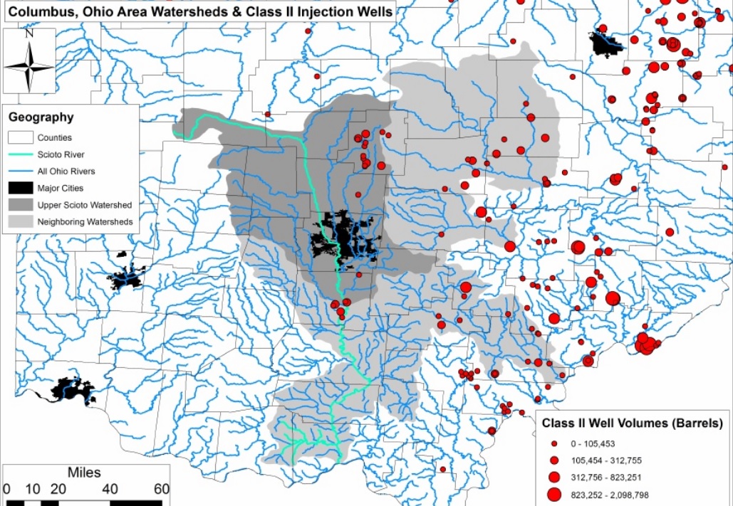
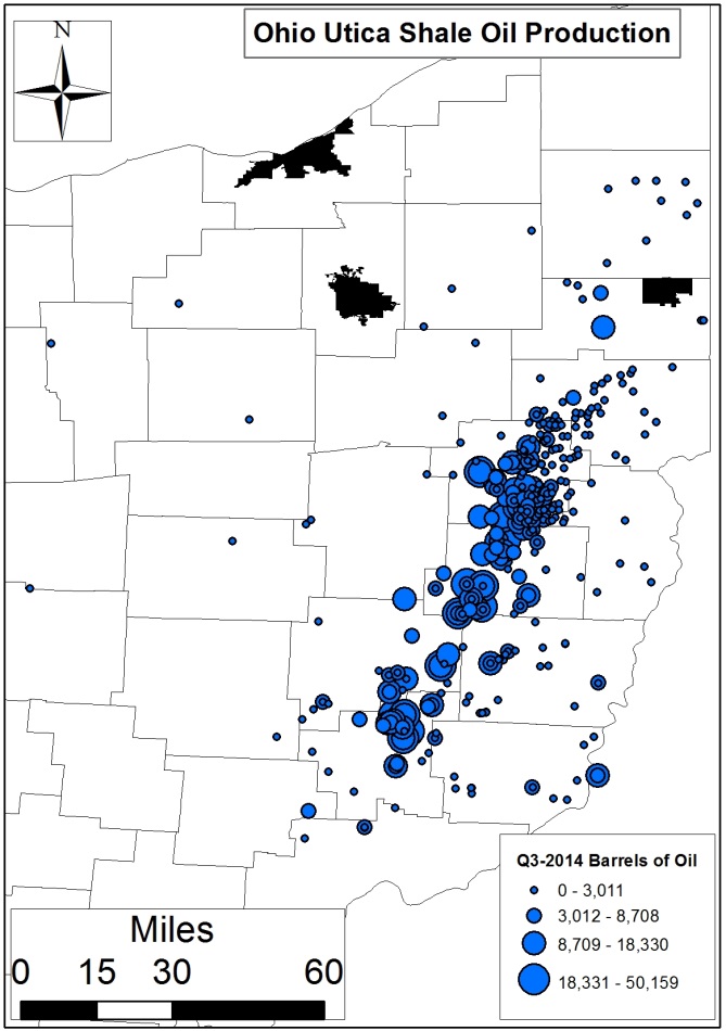
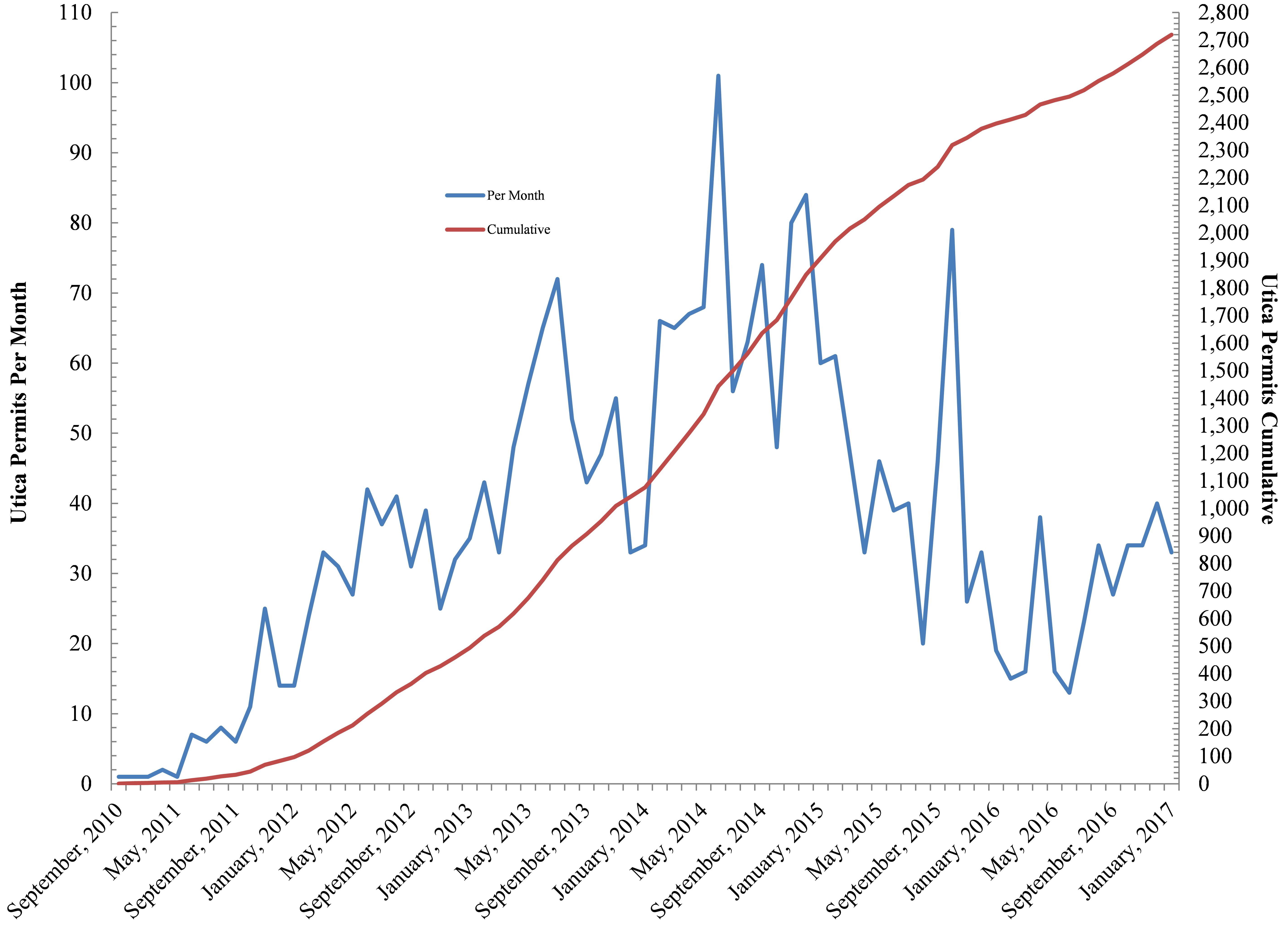
Just how close are public water supplies to Class II waste disposal wells and permitted Utica wells? As of January 15, 2017, there are 13 PWS’s within a half-mile of Ohio’s Class II SWD wells, and 18 within a half-mile of permitted Utica wells. These facilities serve approximately 2,000 Ohioans each, with an average of 112-153 people per PWS (Tables 1 and 5). Within one mile from these wells there are 64 to 66 PWSs serving 18 to 61 thousand Ohioans. That’s an average of 285-925 residents.

Above: Photos of SWD wells from the sky

While PWSs on the 5-mile perimeter of our analysis don’t immediately conjure up water quality/quantity concerns, they may in the future; the rate of Utica and Class II permitting is likely to accelerate under a new White House administration more friendly to industry and averse to enforcing or enhancing regulatory hurdles.

A total of 960 and 699 PWSs are currently within five miles of Ohio Class II and Utica wells. These facilities service roughly 1.5 million and one-half million Ohioans each day, which is ~13% and 4% of the state, respectively. The average PWS within range of Class II wells is 37% to 330 times the average PWS within range of Utica wells.

Roland Marily Kemble Class II Salt Water Disposal Well, Muskingum County, Ohio, Muskingum River Watershed, 39.975, -81.845, 1,984,787 Barrels of Waste Disposed Between 2010 and Q3-2016

Roland Marily Kemble Class II Salt Water Disposal Well, Muskingum County, Ohio, Muskingum River Watershed, 39.975, -81.845, 1,984,787 Barrels of Waste Disposed Between 2010 and Q3-2016

Fifty-eight (58%) to 69% of the PWSs within range of Class II wells are what the Ohio EPA calls Transient Non-Community (TNC) (Table 2). TNC’s are defined by the OH EPA and OH Department of Agriculture as serving[1]:

…at least 25 different persons over 60 days per year. Examples include campgrounds, restaurants and gas stations. In addition, drinking water systems associated with agricultural migrant labor camps, as defined by the Ohio Department of Agriculture, are regulated even though they may not meet the minimum number of people or service connections.

Meanwhile 60-89% of PWS’s in the shadow of Ohio’s permitted Utica wells are of the TNC variety. Even larger percentages of these PWS’s are either Groundwater or Purchased Groundwater types. Most of the PWS’s within the range gradient we looked at are privately owned, with only handful owned by federal or state agencies (Table 6).

Above: Example Class II salt water disposal (SWD) wells in Ohio

Of the 24 hydrologic unit codes (HUCs)/watersheds that contain Class II SWD wells, the lion’s share of PWS’s within the shadow of injection wells are the Tuscarawas, Mahoning, and Walhonding (Table 3). Even the Cuyahoga River, which feeds directly in the Great Lakes, is home to up to 138 PWS’s within 5 miles of Class II SWD wells. Conversely, only 13 HUCs currently contain Ohio’s Utica wells. Like Class II-affected HUCs, we see that the Mahoning, Tuscarawas, and Cuyahoga PSW’s contain most of the PWSs of interest (Table 7).

Conclusion

Watershed security/resilience concerns are growing in Eastern Ohio. Residential and agricultural water demands are increasingly coming into conflict with the drilling industry’s growing freshwater demand. Additionally, as oil and gas drilling uses more water, we will see more brine produced (Figures 1 and 2).

This, in turn, will create more demand – on top of an already exponential trend (Figure 3) – for Ohio’s existing Class II wells from across Northern Appalachia, stretching from Southeast Ohio and West Virginia to North Central Pennsylvania.

An understanding of the links between watershed security, O&G freshwater demand, brine production, and frack waste disposal is even more critical in areas like Southeast Ohio’s Muskingum River Watershed (Figure 4).

A Dynamic Model of Water Demand Between 2000 and 2020 within the Muskingum River Watershed, Southeast Ohio, Kurtz, E. 2015

Figure 4. A Dynamic Model of Water Demand Between 2000 and 2020 within the Muskingum River Watershed, Southeast Ohio, Kurtz and Auch 2015

This is a region of the state where we have seen new water withdrawal agreements like the one below between the Muskingum River Watershed Conservancy District (MWCD) and Antero described in last week’s Caldwell Journal-Leader, Noble County, Ohio:

The [MWCD], which oversees 10 lakes in east central Ohio, approved a second short-term water sale from Seneca Lake last week. The deal, with Antero Resources, Inc., could net the district up to $9,000 a day over about a three month period, and allows Antero to draw up to 1.5 million gallons of water a day during the months of August, September and October for a total of 135 million gallons; less than one percent of the lake’s estimated volume of 14.2 billion gallons. Antero plans to use the water in its fracking operations in the area and will pay $6 per 1000 gallons drawn.

Consol Energy's Cowgill Road Impoundment, Sarahsville, Wills Creek, Noble County, Ohio, 39.8212, -81.4061

Consol Energy’s Cowgill Road Impoundment, Sarahsville, Wills Creek, Muskingum River Watershed, Noble County, Ohio, 39.8212, -81.4061

This agreement will mean an increase in new Class II SWD permits and/or discussion about converting Ohio’s thousands of other Class II wells into SWD wells. What does this change means for communities that have already seen the industry extract the equivalent of nearly 14% – and even 25-80% in several counties – of residential water from their watersheds, only to inject it 6,000+ feet into the state’s geology is unknown? (Figure 5)

It is critical that we establish and frequently revisit the spatial relationship between oil and gas infrastructure the water supplies of Appalachian Ohio. The state of national politics, federal agency oversight and administrations, growing concerns around climate change, and the fact that Southeast Ohio is experiencing more intense and infrequent precipitation events are testaments to that fact. We will be tracking these changes to Ohio’s landscape as they develop. Stay tuned.

Kleese Disposal Class II Salt Water Disposal Well, Trumbull County, Shenango/Mahoning River, 41.244, -80.641, 3,548,104 Barrels of Waste Disposed Between 2010 and Q3-2016

Kleese Disposal Class II Salt Water Disposal well from the sky, Trumbull County, Shenango/Mahoning River, 41.244, -80.641. Data suggest 3,548,104 barrels of waste have been disposed of there between 2010 and Q3-2016.


Supplemental Tables

Public Water and Class II Wells

Table 1. Number of Ohio public water supplies and population served at several intervals from Class II Injection wells

Well Distance (Miles) # Total Population Ave Served Per Well Max People Per Well
0.5 13 1,992 153 (±120) 446
<1 66 60,539 917 (±4,702) 37,456
<2 198 278,402 1,406 (±4,374) 37,456
<3 426 681,969 1,601(±8,187) 148,000
<4 681 1,086,463 1,596 (±8,284) 148,000
<5 960 1,450,865 1,511 (±7,529) 148,000


Table 2. Ohio public water supplies by system type, source, and ownership at several intervals from Class II Injection wells


Well Distance (Miles)

System Type† Source†† Ownership
 

NTNC


TNC


C


G


GP


S


SP


Private


Local


Fed


State

0.5 3 9 1 13 13
<1 11 47 8 65 1 61 5
<2 30 118 50 177 16 5 164 34
<3 76 245 105 385 32 8 351 75
<4 122 392 167 628 40 12 574 106 1
<5 162 564 234 878 30 32 19 823 135 1 1

† NTNC = Non-Transient Non-Community; TNC = Transient Non-Community; C = Community

†† G = Groundwater; GP = Purchased Groundwater; S = Surface Water; SP = Purchased Surface Water


Table 3. Ohio public water supplies by hydrologic unit code (HUC) at several intervals from Class II Injection wells


HUC Name

Well Distance (Miles)
0.5 <1 <2 <3 <4 <5
Ashtabula-Chagrin, 799 1 5 18 18 22
Black-Rocky, 859 1 1 2 2 9
Cuyahoga, 832 1 8 20 92 92 138
Grand, 811 12 30 71 71 81
Hocking, 1081 4 18 18 22
Licking, 1010 1 2 17 17 29
Little Muskingum-Middle Island, 1062 1 2 2 6
Lower Maumee, 856 2 2 4
Lower Scioto, 1091 6 6 9
Mahoning, 831 9 17 48 129 129 161
Mohican, 919 1 3 3 4
Muskingum, 1006 1 3 15 15 33
Raccoon-Symmes, 1128 1
Sandusky, 862 3 19 19 27
Shenango, 815 1 2 6 10 10 11
St. Mary’s, 934 3 5 5 7
Tiffin, 837 4 4 7
Tuscarawas, 889 1 9 76 147 147 213
Upper Ohio, 901 3 15 15 23
Upper Ohio-Shade, 1120 4 8 8 9
Upper Ohio-Wheeling, 984 1 1 4 4 5
Upper Scioto, 959 5 13 13 23
Walhonding, 906 1 11 26 69 69 101
Wills, 1009 2 3 12 12 14


Table 4. Ohio public water supplies by county at several intervals from Class II Injection wells


County

Well Distance (Miles)
0.5 <1 <2 <3 <4 <5
Ashtabula 4 9 16 19 22
Athens 1 2 2 3
Auglaize 3 5 5 7
Belmont 1 4 5 6
Carroll 2 9 20
Columbiana 1 2 6 13 20 32
Coshocton 7 8 10 13
Crawford 1
Cuyahoga 1
Delaware 1
Fairfield 4
Franklin 1 3 7
Fulton 2 4 8
Gallia 1
Geauga 8 19 33 60 71
Guernsey 2 4 10 11 11
Harrison 1 1
Henry 2 3 3
Henry 2 3
Hocking 3 10 11 13
Holmes 1 11 34 25 38 47
Jefferson 1 3 3 5
Knox 2 6 8 9
Lake 1 4 7 17 18
Licking 1 2 10 14 26
Lorain 1 4
Mahoning 3 4 13 25 37 48
Medina 1 1 1 2 5
Meigs 4 5 6 7
Morgan 1 1 1 6 17
Morrow 3 8 11 11
Muskingum 3 8 15
Noble 1 2 2 3
Perry 5 6 8
Pickaway 2 3 7 10
Portage 3 12 41 62 90 113
Seneca 1 12 17 21
Stark 1 4 20 52 121 161
Summit 2 12 26 51
Trumbull 3 7 24 32 45 61
Tuscarawas 6 10 22 24 26
Washington 1 2 4 9
Wayne 1 1 9 18 24 54
Wyandot 2 2 2 3

Public Water and Hydraulically Fractured Wells

Table 5. The number of Ohio public water supplies and population served at several intervals from hydraulically fractured Utica Wells

Well Distance (Miles) # Total Population Ave Served Per Well Max People Per Well
0.5 18 2,010 112 (±72) 31
<1 64 17,879 279 (±456) 2,598
<2 235 116,682 497 (±1,237) 8,728
<3 433 257,292 594 (±2,086) 29,787
<4 572 380,939 666 (±2,404) 29,787
<5 699 496,740 711 (±2,862) 47,348


Table 6. Ohio public water supplies by system type, source, and ownership at several intervals from hydraulically fractured Utica Wells


Well Distance (Miles)

System Type† Source†† Ownership
 

NTNC


TNC


C


G


GP


S


SP


Private


Local


Fed


State

0.5 1 16 1 17 1 18
<1 9 45 10 59 3 1 1 58 6
<2 50 137 48 216 6 3 10 206 29
<3 83 265 85 400 14 5 14 381 51 1
<4 109 352 111 534 16 7 15 504 67 1
<5 141 421 137 652 19 9 18 621 77 1

† NTNC = Non-Transient Non-Community; TNC = Transient Non-Community; C = Community

†† G = Groundwater; GP = Purchased Groundwater; S = Surface Water; SP = Purchased Surface Water


Table 7. Ohio public water supplies by hydrologic unit code (HUC) at several intervals from hydraulically fractured Utica wells


HUC Name

Well Distance (Miles)
0.5 <1 <2 <3 <4 <5
Black-Rocky, 859 1 4 4 4
Cuyahoga, 832 2 12 31 54 82
Grand, 811 1 15 18 23
Licking, 1010 2 2 3 3
Little Muskingum-Middle Island, 1062 2 5 10 11 11
Mahoning, 831 2 5 48 105 142 175
Muskingum, 1006 3 7 9 11
Shenango, 815 2 5 10 13 14
Tuscarawas, 889 8 28 87 140 178 220
Upper Ohio, 901 7 20 45 66 72 73
Upper Ohio-Wheeling, 984 1 13 23 27 28
Walhonding, 906 10 15 34 47
Wills, 1009 2 3 5 7 8


Table 8. Ohio public water supplies by county at several intervals from hydraulically fractured Utica wells


County

Well Distance (Miles)
0.5 <1 <2 <3 <4 <5
Ashtabula 1 1
Belmont 1 2 7 14 15 16
Carroll 6 20 36 43 43 43
Columbiana 4 15 45 72 80 81
Coshocton 7 10 10
Geauga 14 20 25
Guernsey 1 1 2 4 5
Harrison 2 6 16 16 16 16
Holmes 5 13 31 43
Jefferson 2 3 11 22 25 25
Knox 1 1 2 2
Licking 1 1 1 1
Mahoning 2 10 32 44 55
Medina 1 4 5 7
Monroe 2 4 6 6 6
Muskingum 1 1 1 2 3
Noble 2 2 2 2
Portage 2 8 25 49 84
Stark 2 5 40 85 110 122
Summit 6 10
Trumbull 3 23 36 53 65
Tuscarawas 1 2 15 22 28 43
Washington 3 10 12 13
Wayne 5 5 7 21

Footnote

  1. Community (C) = serve at least 15 service connections used by year-round residents or regularly serve at least 25 year-round residents. Examples include cities, mobile home parks and nursing homes; Non-Transient, Non-Community (NTNC) = serve at least 25 of the same persons over six months per year. Examples include schools, hospitals and factories.

By Ted Auch, Great Lakes Program Coordinator, FracTracker Alliance

Power Plants & Other Facilities Now on Ohio Oil & Gas Map

Over the last few months we’ve been busy working on some updates to our Ohio Oil & Gas Map. Check out what we’ve added recently and explore the map below!

New: Power Plants & ATEX Pipeline

We now have the locations of eight of the credible natural gas power plants proposed in Ohio, along with the jobs they cite during construction and operations. We also now have a complete inventory of 118 existing power plants, including 25 natural gas facilities. Together, these plants would produce 7,660 megawatts, around 957 per facility.

Six of these plants are either in the heart of Ohio’s Utica Shale or within several miles of the 1,200+ mile Appalachia-to-Texas (ATEX) pipeline. ATEX was installed to transport 190,000 barrels per day (BPD) of natural gas liquids (NGLs) from the Marcellus and Utica region to the Texas and Louisiana Gulf Goast refinery corridor. The 360 mile segment of this pipeline that runs from Pennsylvania to south central Jackson County, Indiana is also now shown on the Ohio Oil & Gas Map.

Late Permitting Increases

Cumulative and Monthly Ohio Utica Hydraulic Fracturing Well Permits

Figure 1. Cumulative and monthly hydraulic fracturing well permits in Ohio’s Utica Shale

While many shale plays across the United States are experiencing a period of contraction (with low gas prices often cited as the primary reason), drilling activity in Ohio’s Utica Shale has been experiencing a slow and steady expansion. The region has seen more than 2,700 permitted wells as of the end of January 2017. Incidentally, roughly 59% of these wells are producing either oil or gas as of Q3-2016. For more information on that subject, explore our production map.

The permitting trajectory hit a low of 13-16 permits per month between February and January of 2016. Since the presidential election in November, however, permitting rates have more than doubled (Figure 1).

Ohio Oil & Gas Map

Ohio sits on the western edge of both the Utica and Marcellus Shale formations, but conditions are such that the Marcellus Shale is all but being ignored in Ohio. Explore our updated map of OH drilling activity and related facilities below:


View map fullscreen | How FracTracker maps work

Map Layers

The map above is made up of various datasets, from the location of permits to compressor stations. These “map layers” make up the legend. Below we describe each layer on the map, as well as the data source and date range.


Horizontal Marcellus Permits, Laterals
There have been 40+ permits issued for horizontal wells in Ohio’s Marcellus Shale.

Source:   Ohio Department of Natural Resources
Date Range:  December 2009 – Present


Horizontal Utica Permits
An aggregate of ODNR’s monthly cumulative Utica and Marcellus permits as well as a more detailed weekly Risk Based Data Management System (RBDMS) Microsoft Access inventory. At the present time Ohio is home to 2,160+ permitted Utica Wells with the wells broken out by status. Additionally this layer contains depth, water usage, sand usage, HCl, and Gelling Agent percentage for 249 wells based on data provided to FracFocus. Finally, we have incorporated production in various units from individual industry press releases and the ODNR annual report.

Source:   Ohio Department of Natural Resources
Date Range:  December 2009 – Present


Horizontal Utica Permits actual and straight line laterals
An aggregate of ODNR’s monthly cumulative Utica and Marcellus permits as well as a more detailed weekly Risk Based Data Management System (RBDMS) Microsoft Access inventory. At the present time we have straight line laterals for all drilled, drilling, and producing wells as well as actual PLAT laterals for 341 of the wells.

Source:   Ohio Department of Natural Resources
Date Range:  December 2009 – Present


High Volume Hydraulic Fracturing Gathering Lines
All gathering lines servicing Ohio’s inventory of High Volume Hydraulic Fracturing (HVHF) wells.

Source:   Herbert Hoover Foundation grant
Date Range:  December 2009 – 2015


High Volume Hydraulic Fracturing Well Pads
The well-pads of all Ohio’s drilled or producing High Volume Hydraulic Fracturing (HVHF) wells.

Source:   Herbert Hoover Foundation grant
Date Range:  December 2009 – 2015


High Volume Hydraulic Fracturing Well Pad’s Limits Of Disturbance (LOD)
Limits Of Disturbance (LOD) for all Ohio’s drilled or producing High Volume Hydraulic Fracturing (HVHF) well-pads.

Source: Herbert Hoover Foundation grant
Date Range:  December 2009 – 2015


Compressor Stations and Cracking Facilities
Boundaries of several confirmed High Volume Hydraulic Fracturing (HVHF) servicing cracking and compressor station facilities.

Source:   Herbert Hoover Foundation grant
Date Range:  December 2009 – 2015


Ohio Active Class II Injection Wells
This data speaks to the state’s “Active” Class II Injection wells able to accept hydraulic fracturing waste. There are 240+ Active Wells with 51 having yet to receive waste from hydraulic fracturing. For more on Ohio’s Class II Inventory in depth refer to our recent Ohio Fracking Waste Transport & Disposal Network article.

Source:   Ohio Department of Natural Resources
Date Range:  Historical to October, 2015


Earthquakes of >2.0 Magnitude
This data speaks to the state’s 258 earthquakes with current updates from the Ohio Seismic Network and historical quakes – all >2.0 magnitude. These data come from the department’s inventory. Additionally, we present Ohio earthquakes with <2.0 magnitude courtesy of Environment Canada’s Search the Earthquake Database platform.

Source: Ohio Department of Natural Resources, Division of Geological Survey, The Ohio Seismic Network
Date Range:  Historical to Present

AG Pruitt testifies before a congressional committee on issues surrounding energy and the environment

“Polluting Pruitt:” A Wolf to Guard the Hen House?

Guest article by Dakota Raynes, Co-Organizer of Stop Fracking Payne County (OK)

President Trump recently tapped Oklahoma Attorney General Scott Pruitt to head the Environmental Protection Agency (EPA), even though Pruitt is a self-proclaimed “leading advocate against the EPA’s activist agenda.” Pruitt is currently opposing investigation of Exxon Mobile’s handling of climate-change science based on the belief that climate change science is not yet settled and “debate should be encouraged in classrooms, public forums, and the halls of Congress.” Senate confirmation hearings regarding Pruitt’s nomination are currently ongoing – many questions have focused on Pruitt’s legacy as AG of OK and what that tells us about actions he might take as head of the EPA.

Pruitt’s Past as AG

Elected in 2010, Pruitt’s six-year tenure illuminates the full extent of the troubling stances he takes. For instance, he has fought against the overturn of DOMA, same-sex marriage rights, granting legal status to undocumented immigrants, the Affordable Care Act, access to safe and affordable birth control and abortions, and Dodd-Frank Wall Street reform. These actions demonstrate Pruitt’s inability to accept or implement procedures, policies, and programs supported by a majority of US residents, members of the nations’ highest courts, and even his own colleagues.

A Focus on Environmental Issues

More specifically related to environmental issues, he has openly criticized the EPA in congressional hearings and op-ed pieces. Due to his belief that the EPA frequently abuses its authority, Pruitt’s office has filed 14 antiregulatory lawsuits against the EPA. Investigative reporters uncovered that in 13 of these cases co-litigators included companies that had contributed significant amounts of money to Pruitt and/or Pruitt-affiliated political action committees (PACs). He also routinely joins lawsuits against other states. For example, Pruitt and five other Attorneys General challenged a California law banning the sale of eggs laid by hens living in cramped conditions, but a US District Judge ruled they lacked legal standing because they were representing the economic interests of a few industrial egg producers rather than the interests of their broader constituents.

Several such lawsuits are still pending, which legal experts and others claim presents a conflict of interest should Pruitt become the new Director of the EPA. When asked specifically about this issue during Senate confirmation hearings, Pruitt refused to recuse himself from the lawsuits, saying he would leave such a decision up to the EPA’s legal counsel team. Notably, across the course of his six-years as AG, Pruitt’s office has distributed more than 700 news releases announcing the office’s actions, his speeches and public appearances, and efforts to challenge federal regulations. More than 50 of these releases promoted the office’s efforts to sue the EPA, but not once has a release described actions the office has taken to enforce environmental laws or to hold violators accountable for their actions.

Potential Conflicts of Interest

In OK, Pruitt has made many choices, that when viewed together, strongly suggest that his loyalties reside with the industries that have donated hundreds of thousands of dollars to his election campaigns rather than with the people he is sworn to protect. Here is a short list of the most troubling examples:

  • Pruitt’s predecessor had filed suit against Tyson, Cargill, and a number of other poultry producers in OK due to inappropriate disposal of an estimated 300,000 tons of animal waste per year, which was causing toxic algae blooms along the Illinois River. But shortly after his election, Pruitt dropped the case, citing a need for more research. Some have questioned whether his decision was impacted by the fact that the poultry industry had donated at least $40,000 to his campaign that year.
  • He also quickly dismantled the Attorney General’s in-house environmental protection unit, a team of four attorneys and a criminal investigator, and replaced it with the state’s first “federalism unit,” which was created to litigate against overreach by the federal government, mostly the EPA. Pruitt has repeatedly made it clear that he believes states should handle environmental issues, regardless of the fact that environmental issues frequently cause problems that cross geopolitical boundaries such as state lines (OK’s induced seismicity issue1 is a key example, more information about induced seismicity can be found here).
  • In 2013, he created a coalition of 9 Attorneys General, major energy CEOs, and their lawyers and brought them all to OK for a strategizing session regarding how to stop government and citizen responses to the ills of the oil and gas industry; it was an all-expenses paid event funded by Mercatus, a right-wing think tank favored by the Koch brothers.
    1. Notably, the energy industry is Pruitt’s second largest campaign contributor. When he came up for re-election in 2013, he chose Harold Hamm (CEO of Continental Resources, one of the largest oil companies in OK) to co-chair his campaign. Shortly after winning reelection in 2014, Pruitt joined forces with key industry players including Oklahoma Gas and Electric and the Domestic Energy Producers Alliance (chaired by Hamm) to file several antiregulatory lawsuits, which include attempts to block the Clean Power Plan and Waters of the US rule.
    2. Pruitt has also served as leader of the Republican Association of Attorneys General, which has collected at least $4.2 million in donations from fossil-fuel related companies since 2013.
  • Recently, local investigative reporters discovered that Pruitt’s office failed to follow a state law requiring state agencies to disclose spending on outside attorneys. Their examination illuminated that Pruitt has spent more than $1 million on legal fees since FY2012 – a total that does not include costs directly related to lawsuits against the EPA or the Affordable Care Act.

Induced-Seismicity and Wastewater Disposal

OK Map of Recent Earthquakes for Pruitt article

Map of Oklahoma Class II Injection Wells and Volumes 2011 to 2015 (Barrels). Click image to explore a full screen, dynamic map.

Oklahoma recently became the earthquake capital of the world due to a phenomenon referred to as injection-induced seismicity. While OK has not historically been known as a seismically active area, thousands of tremors have shaken the state since the shale gas boom began.

Several researchers have used geospatial analysis to demonstrate how these quakes are caused by the high-pressure injection of oil and gas industry wastes such as the flowback and produced water created by the unconventional oil and gas production process known as hydraulic fracturing. The map above shows where injection wells (tan dots) are located and where earthquakes (green dots) occurred from 2011-2015.

Oklahomans have been harmed by the implicitly pro-fracking stance Pruitt has taken, as evidenced by his lack of action regarding induced seismicity – as well as air, water, and soil contamination due to oil and gas industry activities. Several people, including Johnson Bridgewater (Director of OK Chapter of the Sierra Club) have noted that:

There are various places where the attorney general’s office could have stepped in to fix this overall problem…Its job is to protect citizens. Other states were proactive and took these issues on…[yet] Pruitt has been completely silent in the face of a major environmental problem for the state and its taxpayers.

Specifically, the AG’s office could have responded to the legal question of whether the state could limit or ban transport of fracking-related wastewater, sent by other states for disposal in underground injection wells in OK.

He also did nothing to address the phenomenally low earthquake insurance claim approval rate; after the 5.8M quake shook Pawnee in September of 2016, 274 earthquake damage claims were filed but only 4 paid out. Estimates of statewide approval rates generally suggest that approximately 1% of claimants receive funds to aid repairs.

Lastly, there are a number of class action lawsuits against a variety of industry actors regarding earthquake damages, yet Pruitt’s office has not entered any of these as an intervenor even though AGs in other states have done so.

Pruitt not at fault?

Photo Credit: JIM BECKEL/The Oklahoman

Earthquake damage. Photo Credit: Jim Beckel/The Oklahoman

Pruitt was recently called out by investigative reporters who used open-records requests to reveal that letters, briefs, and lawsuits that he submitted were written in whole or in part by leading energy firms such as Devon (another of OK’s largest oil and gas companies). Pruitt’s response was that he had done nothing wrong, nothing even potentially problematic. Rather, he said, of course he was working closely with industry and isn’t that what he should be doing. Some would argue that as AG what he should be doing is working closely with the people of Oklahoma, especially those whose homes, lives, and livelihoods have crumbled under the weight of attempting to repair earthquake damage due to industry activities.

Historical AG Influence

It is important to remember, though, that what’s happening with Pruitt is not isolated. Rather, as several long-time reporters have noted, increased attention to developing beneficial relationships with AGs is a result of historical processes.

About 20 years ago more than 40 state AGs banded together to challenge the tobacco industry, which led to a historic $206 billion settlement decision. Later, Microsoft, the pharmaceutical industry, and the financial services industry each faced similar multistate challenges regarding the legality or illegality of particular business practices.

As some AGs began hiring outside law firms to investigate and sue corporations, industry leaders realized that AGs’ actions were far more powerful and immediate than those of legislative bodies. So, they began a heretofore unprecedented campaign to massively increase their influence at this level.

Several people have critiqued the ways in which such actions undermine democratic processes, prompt troubling questions about ethics, and negatively impact attorney generals’ abilities to fulfill their duties to the state and its residents.

A Mission at Risk

Those of us on the frontlines here in OK have seen just how powerful such coalitions can be, how much sway they can have on local and state officials, how they destabilize people’s faith and trust in the systems that are supposed to protect them, and how coalitions undercut people’s hope and desire to be civically engaged. The mission of the US Environmental Protection Agency is to protect human health and the environment. If confirmed to lead the EPA, it is very likely Pruitt will prioritize his relationships with industry over the health and welfare of the people and environment he’s directed to protect.

Footnotes

  1. To learn more about induced seismicity read an exclusive FracTracker two-part series from former VTSO researcher Ariel Conn: Part I and Part II. Additionally, the USGS has created an Induced Earthquakes landing page as part of their Earthquake Hazards Program.

Hypothetical Impacts of Unconventional Drilling In Allegheny County

With tens of thousands of wells scattered across the countryside, Southwestern Pennsylvania is no stranger to oil and gas development. New, industrial scale extraction methods are already well entrenched, with over 3,600 of these unconventional wells drilled so far in that part of the state, mostly from the well known Marcellus Shale formation.

Southwestern Pennsylvania is also home to the Pittsburgh Metropolitan Area, a seven county region with over 2.3 million people. Just over half of this population is in Allegheny County, where unconventional drilling has become more common in recent years, along with all of its associated impacts. In the following interactive story map, the FracTracker Alliance takes a look at current impacts in more urban and suburban environments, plus projects what future impacts could look like, based on leasing activity.

hypothetical impacts map

By Matt Kelso, Manager of Data & Technology

You Are Here feature image

You Are Here!

Oklahoma and Kansas Class II Injection Wells and Earthquakes

By Ted Auch, Great Lakes Program Coordinator, FracTracker Alliance
In collaboration with Caleb Gallemore, Assistant Professor in International Affairs, Lafayette University

The September 3rd magnitude 5.8 earthquake in Pawnee, Oklahoma, is the most violent example of induced seismicity, or “man-made” earthquakes, in U.S. history, causing Oklahoma governor Mary Fallin to declare a state of emergency. This was followed by a magnitude 4.5 earthquake on November 1st prompting the Oklahoma Corporation Commission (OCC) and U.S. EPA to put restrictions on injection wells within a 10-mile radius of the Pawnee quake.

And then on Sunday, November 6th, a magnitude 5.0 earthquake shook central Oklahoma about a mile west of the Cushing Hub, the largest commercial crude oil storage center in North America capable of storing 54 million barrels of crude. This is the equivalent of 2.8 times the U.S. daily oil refinery capacity and 3.1 times the daily oil refinery capacity of all of North America. This massive hub in the North American oil landscape also happens to be the southern terminus of the controversial Keystone pipeline complex, which would transport 590,000 barrel per day over more than 2,000 miles (Fig. 1). Furthermore, this quake demonstrated the growing connectivity between Class II injection well associated induced seismicity and oil transport/storage in the heart of the US version of Saudi Arabia’s Ghawar Oil Fields. This increasing connectivity between O&G waste, production, and processing (i.e., Hydrocarbon Industrial Complex) will eventually impact the wallets of every American.

North American Oil Refinery Capacity, Pipelines, and Cushing, OK

Figure 1. The Keystone Pipeline would transport 590,000 bpd over more than 2,000 miles.

This latest earthquake caused Cushing schools to close. Magellan Midstream Partners, the major pipeline and storage facility operator in the region, also shut down in order to “check the integrity of our assets.” Compounding concerns about induced seismicity, the Cushing Hub is the primary price settlement point for West Texas Intermediate that, along with Brent Crude, determines the global price of crude oil and by association what Americans pay for fuel at the pump, at their homes, and in their businesses.

Given the significant increase in seismic activity across the U.S. Great Plains, along with the potential environmental, public health, and economic risks at stake, we thought it was time to compile an inventory of Class II injection well volumes. Because growing evidence points to the relationship between induced seismicity and oil and gas waste disposal, our initial analysis focuses on Oklahoma and Kansas. The maps and the associated data downloads in this article represent the first time Class II injection well volumes have been compiled in a searchable and interactive fashion for any state outside Ohio (where FracTracker has compiled class II volumes since 2010). Oklahoma and Kansas Class II injection well data are available to the public, albeit in disparate formats and diffuse locations. Our synthesis makes this data easier to navigate for concerned citizens, policy makers, and journalists.

Induced Seismicity Past, Present, and Future

inducedseismicity_figure

Figure 2. Central U.S. earthquakes 1973-August 15, 2015 according to the U.S. Geological Survey (Note: Based on our analysis this exponential increasing earthquakes has been accompanied by a 300 feet per quarter increase in the average depth of earthquakes across Oklahoma, Kansas, and Texas).

Oklahoma, along with Arkansas, Kansas, Ohio, and Texas, is at the top of the induced seismicity list, specifically with regard to quakes in excess of magnitude 4.0. However, as the USGS and Virginia Tech Seismological Observatory (VTSO)[1] have recently documented, an average of only 21 earthquakes of magnitude 3.0 or greater occurred in the Central/Eastern US between 1973 and 2008. This trend jumped to an average of 99 between 2009 and 2013. In 2014 there were a staggering 659 quakes. The exponential increase in induced seismic events can be seen in Figure 2 from a recent USGS publication titled “High-rate injection is associated with the increase in U.S. mid-continent seismicity,” where the authors note:

“An unprecedented increase in earthquakes in the U.S. mid-continent began in 2009. Many of these earthquakes have been documented as induced by wastewater injection…We find that the entire increase in earthquake rate is associated with fluid injection wells. High-rate injection wells (>300,000 barrels per month) are much more likely to be associated with earthquakes than lower-rate wells.”

hydraulic-fracturing-freshwater-demand

Figure 3. Average freshwater demand per hydraulically fractured well across four U.S. shale plays and the annual percent increase in each of those plays.

This trend suggests that induced seismicity is the new normal and will likely increase given that: 1) freshwater demand per hydraulically fractured well is rising all over the country, from 11-15% per year in the Marcellus and Bakken to 20-22% in the Denver and Midland formations, 2) the amount of produced brine wastewater parallels these increases almost 1-to-1, and 3) the unconventional oil and gas industry is using more and more water as they begin to explore the periphery of primary shale plays or in less productive secondary and tertiary plays (Fig. 3).

Oklahoma

The September, 2016, Pawnee County Earthquake

This first map focuses on the September, 2016 Pawnee, OK Magnitude 5.8 earthquake that many people believe was caused by injecting high volume hydraulic fracturing (HVHF) waste into class II injection wells in Oklahoma and Kansas. This map includes all Oklahoma and Kansas Class II injection wells as well as Oklahoma’s primary geologic faults and fractures.

Oklahoma and Kansas Class II injection wells and geologic faults


View map fullscreenHow FracTracker maps work

Pawnee, Oklahoma 5.8 magnitude earthquake, September, 2016 & Active Class II Injection Wells

Figure 4. The September, 2016 Pawnee, Oklahoma 5.8M earthquake, neighboring active Class II injection wells, underlying geologic faults and fractures.

Of note on this map is the geological connectivity across Oklahoma resulting from the state’s 129 faults and fractures. Also present are several high volume wells including Territory Resources LLC’s Oldham #5 (1.45 miles from the epicenter, injecting 257 million gallons between 2011 and 2014) and Doyle #5 wells (0.36 miles from the epicenter, injecting 61 million gallons between 2011 and 2015), Staghorn Energy LLC’s Hudgins #1 well (1.43 miles from the epicenter, injecting 11 million gallons between 2011 and 2015 into the Red Fork formation), and Cooke Co Production Co.’s Laird #3-35 well (1.41 miles from the epicenter, injecting 6.5 million gallons between 2011 and 2015). Figure 4 shows a closeup view of these wells relative to the location of the Pawnee quake.

Class II Salt Water Disposal (SWD) Injection Well Volumes

This second map includes annual volumes of disposed wastewater across 10,297 Class II injection wells in Oklahoma between 2011 and 2015 (Note: 2015 volumes also include monthly totals). Additionally, we have included Oklahoma’s geologic faults and fractures for context given the recent uptick in Oklahoma and Kansas’ induced seismicity activity.

Annual volumes of class II injection wells disposal in Oklahoma (2011-2015)


View map fullscreenHow FracTracker maps work | Download map data

Oklahoma statistics for 2011 to 2015 (Table 1):

  1. Maximum volume to date (for a single Class II injection well): 105,979,598 barrels, or 4,080,214,523 gallons (68,003,574 gallons per month), for the New Dominion, LLC “Chambers #1” well in Oklahoma County.
  2. Total Volume to Date: 10,655,395,179 barrels or 410,232,714,392 gallons (6,837,211,907 gallons per month).
  3. Mean volume to date across the 10,927 Class II injection wells: approximately 975,144 barrels per well or 37,543,044 gallons (625,717 gallons per month).
  4. This map also includes 632 Class II wells injecting waste into the Arbuckle Formation which is believed to be the primary geological formation responsible for the 5.0 magnitude last week in Cushing.

Kansas

Below is an inventory of monthly oil and gas waste volumes (barrels) disposed across 4,555 Class II injection wells in Kansas between 2011 and 2015. This map will be updated in the Spring of 2017 to include 2016 volumes. A preponderance of this data comes from 2015 with a scattering of volume reports across Kansas between 2011 and 2014.

Monthly Class II injection wells volumes in Kansas (2011-2015)


View map fullscreenHow FracTracker maps work | Download map data

Kansas statistics for 2015 (Table 1):

  1. Maximum volume to date (for a single Class II injection well): 9,016,471 barrels, or 347,134,134 gallons (28,927,845 gallons per month), for the Sinclair Prairie Oil Co. “H.J. Vohs #8” well in Rooks County. This is a well that was initially permitted and completed between 1949 and 1950.
  2. Total Volume to date: 1,060,123,330 barrels or 40,814,748,205 gallons (3,401,229,017 gallons per month).
  3. Mean volume to date across the 4,555 Class II injection wells: approximately 232,738 barrels per well or 8,960,413 gallons (746,701 gallons per month).

Table 1. Summary of Class II SWD Injection Well Volumes across Kansas and Oklahoma


Sum Average Maximum
No. of Class II
SWD Wells
Barrels Sum To Date Per Year Sum To Date Per Year
Kansas* 4,555 1.06 BB 232,738 9.02 MB
Oklahoma** 10,927 10.66 BB 975,143 195,029 105.98 MB 21.20 MB

* Wells in the counties of Barton (279 wells), Ellis (397 wells), Rooks (220 wells), Russell (199 wells), and Ness (187 wells) account for 29% of Kansas’ active Class II wells.

** Wells in the counties of Carter (1,792 wells), Creek (946 wells), Pontotoc (684 wells), Seminole (476 wells), and Stephens (1,302 wells) account for 48% of Oklahoma’s active Class II wells.

Conclusion

If the U.S. EPA’s Underground Injection Control (UIC) estimates are to be believed, the above Class II volumes account for 19.3% of the “over 2 billion gallons of brine…injected in the United States every day,” and if the connectivity between injection well associated induced seismicity and oil transport/storage continues to grow, this issue will likely impact the lives of every American.

Given how critical the Cushing Hub is to US energy security and price stability one could easily argue that a major accident there could result in a sudden disruption to fuel supplies and an exponential increase in “prices at the pump” that would make the 240% late 1970s Energy Crisis spike look like a mere blip on the radar. The days of $4.15 per gallon prices the country experienced in the summer of 2008 would again become a reality.

In sum, the risks posed by Class II injection wells and are not just a problem for insurance companies and residents of rural Oklahomans and Kansans, induced seismic activity is a potential threat to our nation’s security and economy.

Downloads

FracTracker Induced Seismicity Infographic (print quality)

Oklahoma Class II SWD Injection Well Annual Volumes 2011 to 2015 (Barrels)

Kansas Class II SWD Injection Well Monthly Volumes 2011 to 2015 (Barrels)

Footnotes

[1] To learn more about Induced Seismicity read an exclusive FracTracker two-part series from former VTSO researcher Ariel Conn: Part I and Part II. Additionally, the USGS has created an Induced Earthquakes landing page as part of their Earthquake Hazards Program.