Groundwater Threats in Colorado
FracTracker has been increasingly looking at oil and gas drilling in Colorado, and we’re finding some interesting and concerning issues to highlight. Firstly, operators in Colorado are not required to report volumes of water use or freshwater sources. Additionally, this analysis looked at how wastewater in Colorado is injected, and found that the majority is injected into Class II disposal wells (85%) while recycling wastewater is not common. Open-air pits for evaporation and percolation of wastewater is still a common practice. Colorado has at least 340 zones granted aquifer exemptions from the Clean Water Act for injecting wastewater into groundwater. The analysis also found that Weld County produces the most oil and gas in the state, while Rio Blanco and Las Animas counties produce more wastewater. And finally, Rio Blanco injects the most wastewater of all Colorado counties. Learn more about groundwater threats in Colorado below:
Introduction
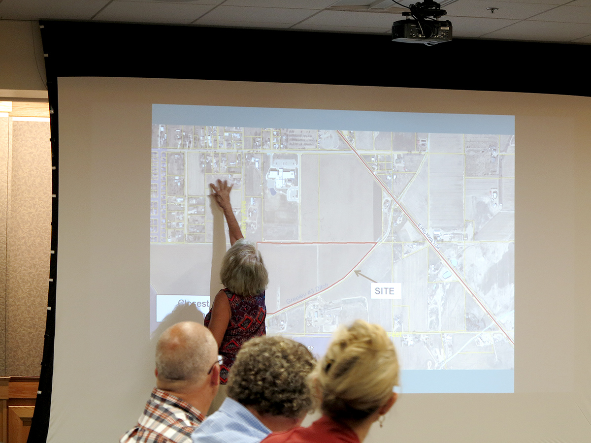
Working directly with communities in Weld County, Colorado the FracTracker Alliance has identified issues concerning oil and gas exploration and production in Colorado that are of particular concern to community stakeholder groups. The issues include air quality degradation, environmental justice concerns for communities most impacted by oil and gas extraction, and leasing of federal mineral estates. Analysis of data for Colorado’s Front Range has identified areas where setback regulations are not followed or are inadequate to provide sufficient protections for individuals and communities and our analysis of floodplains shows where oil and gas operations pose a significant risk to watersheds. In this article we focus on the specific threat to groundwater resources as a result of particular waste disposal methods, namely underground injection and land application in disposal pits and sumps. We also focus on the sources of the immense amount of water necessary for fracking and other extraction processes.
Groundwater Threats
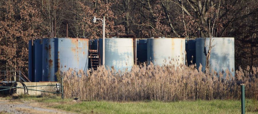
Numerous threats to groundwater are associated with oil and gas drilling, including hydraulic fracturing. Research from other regions shows that the majority of groundwater contamination events actually occur from on-site spills and poor management and disposal of wastes. Disposal and storage sites and spill events can allow the liquid and solid wastes to leach and seep into groundwater sources. There have been many groundwater contamination events documented to have occurred in this manner. For example, in 2013, flooding in Colorado inundated a main center of the state’s drilling industry causing over 37,380 gallons of oil to be spilled from ruptured pipelines and damaged storage tanks that were located in flood-prone areas. There are serious concerns that the oil-laced floodwaters have permanently contaminated groundwater, soil, and rivers.
Waste Management
In Colorado, wastes are managed several ways. If the wastewater is not recycled and used again in other production processes such as hydraulic fracturing, drilling fluids disposal must follow one of three rules:
- Treated at commercial facilities and discharged to surface water,
- Injected in Class II injection wells, or
- Stored and applied to the land and disposal pits at centralized exploration and production waste management facilities.
Additionally the wastes can be dried and buried in additional drilling pits, with restrictions for crop land. For oily wastes, those containing crude oil, condensate or other “hydrocarbon-containing exploration and production waste,” there are additional land application restrictions that mostly require prior removal of free oil. These various sites and facilities are mapped below, along with aquifer exemptions and other map layers related to water quality.
Figure 1. Interactive map of groundwater threats in Colorado
View Map Fullscreen | How Our Maps Work
Injection Wells
In 2015, Colorado injected a total of 649,370,514 barrels of oil and gas wastewater back into the ground. That is 27,273,561,588 gallons, which would fill over 41,000 Olympic sized swimming pools. Injected into the ground in deep formations, this water is forever removed from the water cycle.
Allowable injection fluids include a variety of things you do not want to drink:
- Produced Water
- Drilling Fluids
- Spent Well Treatment or Stimulation Fluids
- Pigging (Pipeline Cleaning) Wastes
- Rig Wash
- Gas Plant Wastes such as:
- Amine
- Cooling Tower Blowdown
- Tank Bottoms
This means that federal exemptions to Underground Injection Control (UIC) regulations for oil and gas exploration and production have nothing to do with environmental chemistry and risk, and only consider fluid source.
Why the concern?
Why are we concerned about these wastes? To quote the regulation, “it is possible for an exempt waste and a non-exempt hazardous waste to be chemically very similar” (RCRA). Since oil and gas development is considered part of the United State’s strategic energy policy, the entire industry is exempt from many federal regulations, such as the Safe Drinking Water Act (SDWA), which protects underground sources of drinking water (USDW).
The Colorado Oil and Gas Conservation Commission has primacy over the UIC permits and the Colorado Department of Public Health and Environment (CDPHE) administers the environmental protection laws related to air quality, waste discharge to surface water, and commercial disposal facilities. Under the UIC program, operators are legally allowed to inject wastewater containing heavy metals, hydrocarbons, radioactive elements, and other toxic and carcinogenic chemicals into groundwater aquifers.
The State of CO Injection Wells
According to the COGCC production reports for the year 2015, there are 9,591 active injection wells with volumes reported to the regulatory agency. Additionally, there are of course distinctions within the UIC rules for different types of injection wells, although the COGCC does not provide comprehensive data to distinguish between these types.
Injecting into the same geological formation or “zone” as producing wells is typically considered EOR, although some of the injected water will ultimately remain in the ground. Injecting into a producing formation is an immediate qualification for receiving an aquifer exemption.
EOR operations require considerably more energy and resources than conventional wells, and therefore have a higher water carbon footprint. If the wastewater is “recycled” as hydraulic fracturing fluid, the injections are exempt from all UIC regulations regardless. These are two options for the elimination of produced wastewater, although much of it will return to the surface in the future along with other formation waters. When the produced waters reach a certain level of salinity the fluid can no longer be used in enhanced recovery or stimulation, so final disposal of wastewater is typically necessary. These liquid wastes may then go to UIC Class II Disposal Wells.
Class II Injection Wells
The wells injecting into non-producing formations are therefore disposal wells, since they are not “enhancing production.” Of the almost 10,000 active injection wells in Colorado there are OVER 670 class II disposal well facilities; 402 facilities are listed as currently active. These facilities may or may not host multiple wells. By filtering the COGCC production and injection well database by target formation, we find that there are over 1,070 wells injecting into non-producing formations. These disposal wells injected at least 66,193,874 barrels (2,780,142,708 gallons) of wastewater in 2015 alone.
Where is the waste going?
A simple life-cycle assessment of wastewater in Colorado shows that the majority of produced water is injected back underground into class II disposal and EOR wells. The percentage of injected produced waters has been increasing since 2012, and in 2015 85% of the total volume of produced water in 2015 was injected.
If we assume that all the volume injected was produced wastewater, this still leaves 60 million barrels of produced water unaccounted for. Some of this volume may have been recycled and used for hydraulic fracturing, but this is rarely the case. Other options for disposal include commercial oilfield wastewater disposal facilities (COWDF) that use wastewater sumps (pits) for evaporation and percolation, as well as land application, to dilute the solid and liquid wastes by mixing them into soil.
Centralized Exploration and Production Waste Management Facilities
Figure 2. Chevron Wastewater Land Application and Pit “Disposal” Facility. Photo by COGCC
According to the COGCC, there are 40 active and 71 total “centralized exploration and production waste management facilities” in Colorado. These facilities, mapped in Figure 1 above, are mostly open-air pits used for storage or disposal, or land-application sites.
As can be seen in the Figure 2 to the right, land application sites are little more than farms that don’t grow anything, where wastewater is mixed with soil. Groundwater monitoring wells around these sites measure the levels of some contaminants. Inspection reports show that sampling of the wastewater is not usually – if ever – conducted. The only regulatory requirement is that oil is not visibly noticeable as a sheen on the wastewater fluids in impoundments, such as the one in Figure 3 below, operated by Linn Operating Inc., which is covered in an oily sheen.
In most other hydrocarbon producing states, open-air pits or sumps are not allowed for a variety of reasons. At FracTracker, we have covered this issue in other states, as well. In New Mexico, for example, the regulatory agency outlawed the use of pits after finding cased where 369 pits were documented to have contaminated groundwater. California is another state that still uses above ground pits for disposal. At sites in California, plumes of contaminants are being monitored as they spread from the facilities into surrounding regions of groundwater. Additionally, these wastewater pit disposal sites present hazards for birds and wildlife. There have been a number of papers documenting bird deaths in pits, and the risk for migratory bird species is of high concern. Other states like California are struggling with the issue of closing these types of open-air pit facilities. Closing these facilities means that more wastewater will be injected in Class II disposal wells.
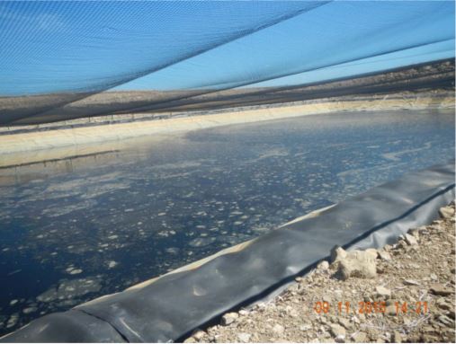
Figure 3. Linn energy oily wastewater disposal pit
Production and Injection Volumes
The data published by the COGCC for well production and injection volumes shows some unique trends. An analysis of injection and production well volumes shows Class II Injection is tightly connected to exploration and production activities. This finding is not surprising. Class II injection wells are considered a support operation for the production wells, and therefore should be expected to be similarly related. Wastewater injection wells are needed where oil and gas extraction is occurring, particularly during the exploration and drilling phases.
Looking at the graphs in Figures 4-6 below, it is obvious that injection volumes have been consistently tied to production of wastewater. It is also clear that the trend since 2012 shows that an increasingly larger percentage of wastewater is being injected each year. This trend follows the sharp increase in high volume hydraulic fracturing activity that occurred in 2012. During this boom in exploration and drilling activity, recycling of flowback for additional hydraulic fracturing activities most likely accounts for some of the discrepancy in accounting for the fact that 200% more wastewater was produced than was injected in 2012.
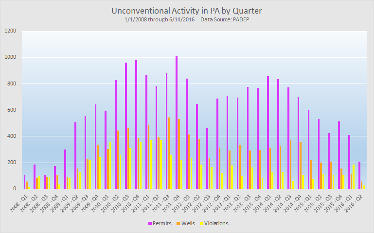
When Figure 4 (below) is compared to the graphs in Figures 5 and 6 (further below) it is also interesting to note that produced water volumes in 2015 are at a 5-year low as of 2015, while production volumes of both natural gas and oil are at a 5-year high. Wastewater volumes are linked to production volumes, but there are many other factors, including geological conditions and types of extraction technologies being used, that have a massive affect on wastewater volumes.
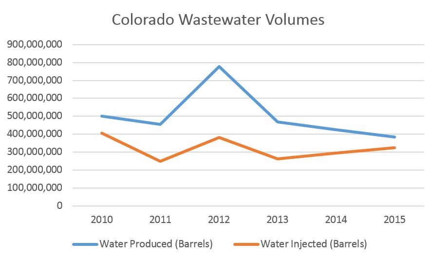
Figure 4. Colorado wastewater volumes by year (barrels)
The graphs in Figures 5 and 6 below show different trends. Gas production in Colorado has remained relatively constant over the last five years with a sharp increase in 2015, while oil production volumes have been continually increasing, with the largest increase of 49% from 2014 to 2015, and 46% the year prior.
Figures 5-6


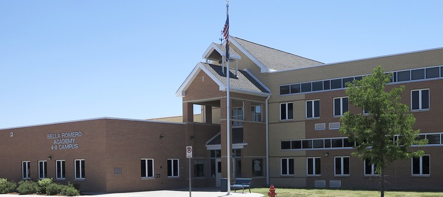
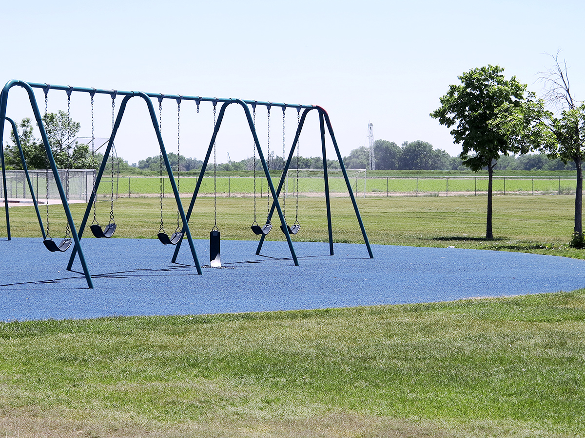
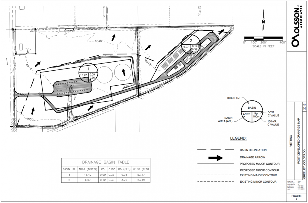
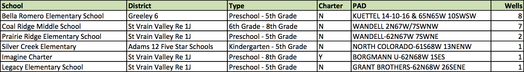
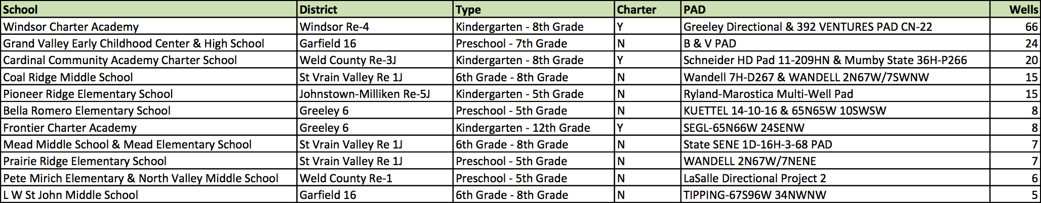
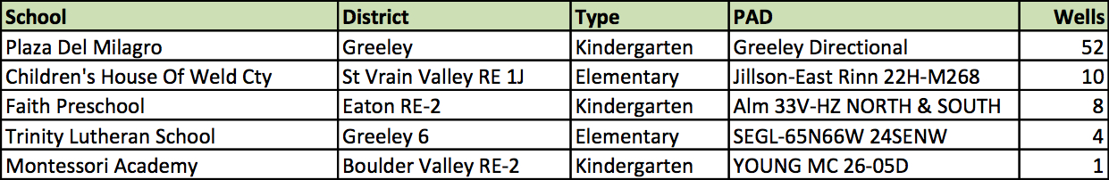
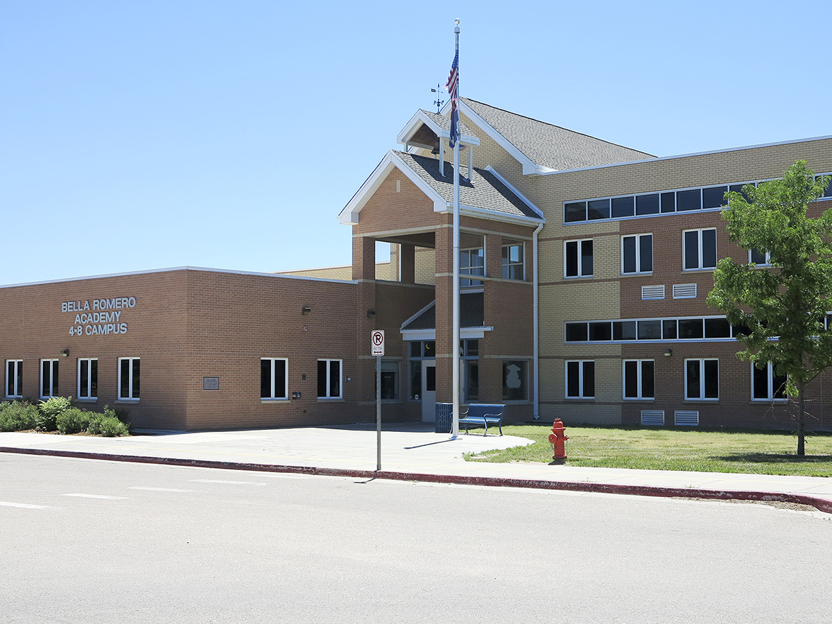
Colorado’s Front Range, specifically Weld County, is increasing oil production at a fast rate. New multi-well well-pads are being permitted in neighborhoods and urban and suburban communities without consideration for even elementary schools. Weld County currently has 2,169 new wells permitted within the county. The figure is higher than the next 9 counties combined. The other top three counties with the most well permits are 2. Garfield (1,130) and 3. Rio Blanco (189), for perspective. Additionally, 74% of pending permits for new wells are located in Weld County.
How Counties Compare
The top 10 counties for oil production are very similar to the top 10 counties for both produced and injected volumes, although there are some inconsistencies (Table 1). For example, Las Animas County produces the second largest amount of produced wastewater, but is not in the top 10 of oil producing counties. This is because the majority of wells in Las Animas County produce natural gas. Natural gas wells do not typically produce as much wastewater as oil wells. The counties and areas with the most oil and gas production are also the regions with the most injection and surface waste disposal, and therefore surface water and groundwater degradation.
Table 1. Top 10 CO counties for gas production, oil production, wastewater production, and injection volumes in 2015.
| Gas Production | Oil Production | Wastewater Production | Injection Volumes | |||||
| Rank | County | Gas1 | County | Oil2 | County | Water2 | County | Water2 |
| 1 | Weld | 568,919,168 | Weld | 112,898,400 | Rio Blanco | 113,132,037 | Rio Blanco | 138,502,742 |
| 2 | Garfield | 556,855,359 | Rio Blanco | 4,412,578 | Las Animas | 45,868,907 | Weld | 50,360,796 |
| 3 | La Plata | 322,029,940 | Gardield | 1,744,900 | Weld | 37,665,571 | Garfield | 29,022,147 |
| 4 | Las Animas | 78,947,042 | Araahoe | 1,661,204 | Garfield | 34,704,673 | La Plata | 23,211,646 |
| 5 | Rio Blanco | 57,284,876 | Lincoln | 1,194,435 | Washington | 25,075,998 | Washington | 15,105,886 |
| 6 | Mesa | 32,200,936 | Cheyenne | 1,192,162 | La Plata | 23,352,861 | Las Animas | 13,706,555 |
| 7 | Yuma | 25,960,947 | Adams | 664,530 | Cheyenne | 9,326,944 | Cheyenne | 10,309,413 |
| 8 | Archuleta | 13,648,006 | Moffat | 419,893 | Moffat | 7,712,323 | Logan | 5,930,937 |
| 9 | Moffat | 13,610,219 | Washington | 413,603 | Logan | 5,606,828 | Mesa | 5,611,075 |
| 10 | Gunnison | 4,805,541 | Jackson | 407,537 | Morgan | 4,197,849 | La Plata | 4,992,391 |
| 1. Units are in MCF = Thousand cubic feet of natural gas; 2. Units are in Barrels |
||||||||
Aquifer Exemptions
Operators are given permission by the U.S. EPA to inject wastewater into groundwater aquifers in certain locations where groundwater formations are particularly degraded or when operators are granted aquifer exemptions. Aquifer exemptions are not regions where the groundwater is not suitable for use as drinking water. Quite the contrary, as any aquifer with groundwaters above a 10,000 ppm total dissolved solids (TDS) threshold are fast-tracked for injection permits. When the TDS is below 10,000 ppm operators can apply for an exemption from SDWA (safe drinking water act) for USDWs (underground sources of drinking water), which otherwise protects these groundwater sources. An exemption can be granted for any of the following three reasons. The formation is:
- hydrocarbon producing,
- too deep to economically access, or
- too “contaminated” to economically treat.
Since the first requirement is enough to satisfy an exemption, most class II wells are located within oil and gas fields. Other considerations include approval of mineral owners’ permissions within ¼ mile of the well. On the map above, you can see the ¼ mile buffers around active injection wells. If you live in Colorado, and suspect you live within the ¼ mile buffer of an injection well, you can input an address into the search field in the top-right corner of the map to fly to that location.
Sources of Water
The economic driver for increasing wastewater recycling is mostly influenced by two factors. First, states with many class II disposal wells, like Colorado, have much lower costs for wastewater disposal than states like Pennsylvania, for example. Additionally, the cost of water in drought-stricken states makes re-use more economically advantageous.
These two factors are not weighted evenly, though. On the Colorado front range, water scarcity should make recycling and reuse of treated wastewater a common practice. The stress of sourcing fresh water has not yet become a finanacial restraint for exploration and production. Water scarcity is an issue, but not enough to motivate operators to recycle. According to an article by Small, Xochitl T (2015) “Geologic factors that impact cost, such as water quality and availability of disposal methods, have a greater impact on decisions to recycle wastewater from hydraulic fracturing than water scarcity.” As long as it is cheaper to permit new injection wells and contaminate potential USDW’s than to treat the wastewater, recycling practices will be largely ignored. Even in Colorado’s arid Front Range where the demand for freshwater frequently outpaces supply, recycling is still not common.
Fresh Water Use
The majority of water used for hydraulic fracturing is freshwater, and much of it is supplied from municipal water systems. There are several proposals for engineering projects in Colorado to redirect flows from rivers to the specific municipalities that are selling water to oil and gas operators. These projects will divert more water from the already stressed watersheds, and permanently remove it from the water cycle.
The Windy Gap Firming Project, for example, plans to dam the Upper Colorado River to divert almost 10 billion gallons to six Front Range cities including Loveland, Longmont, and Greeley. These three cities have sold water to operators for fracking operations. Greeley in particular began selling 1,500 acre-feet (500 million gallons) to operators in 2011 and that has only increased . The same thing is happening in Fort Lupton, Frederick, Firestone, and in other communities. Additionally, the Northern Integrated Supply Project proposes to drain an additional 40,000 acre feet/year (13 billion gallons) out of the Cache la Poudre River northwest of Fort Collins. The Seaman Reservoir Project by the City of Greeley on the North Fork of the Cache la Poudre River proposes to drain several thousand acre feet of water out of the North Fork and the main stem of the Cache la Poudre. And finally, the Flaming Gorge Pipeline would take up to 250,000 acre feet/year (81 billion gallons) out of the Green and Colorado Rivers systems, among others.
Other Water Sources
Unfortunately, not much more is known about sources and amounts of water for used for fracking or other oil and gas development operations. Such a data gap seems ridiculous considering the strain on freshwater sources in eastern Colorado and the Front Range, but regulators do not require operators to obtain permits or even report the sources of water they use. Legislative efforts to require such reporting were unsuccessful in 2012.
Now that development and fracking operations are continuously moving into urban and residential areas and neighborhoods, sourcing water will be as easy as going to the nearest fire hydrant. Allowing oil and gas operators to use municipal water sources raises concerns of conflicts of interest and governmental corruption considering public water systems are subsidized by local taxpayers, not well sites.
Conclusions
In Colorado, exploration and drilling for oil and natural gas continues to increase at a fast pace, while the increase in oil production is quite staggering. As this trend continues, the waste stream will continue to grow with production. This means more Class II injection wells and other treatment and disposal options will be necessary.
While other states are working to end the practices that have a track record of surface water and groundwater contamination, Colorado is issuing new permits. Colorado has issued 7 permits for CEPWMF’s in 2016 alone, some of them renewals. While there aren’t any eco-friendly methods of dealing with all the wastewater, the use of pits and land application presents high risk for shallow groundwater aquifers. In addition, sacrificing deep groundwater aquifers with aquifer exemptions is not a sustainable solution. These are important considerations beyond the obvious contribution of carbon dioxide and methane to the issue of climate change when considering the many reasons why hydrocarbon fuels need to be eliminated in favor of clean energy alternatives.
By Kyle Ferrar, Western Program Coordinator & Kirk Jalbert, Manager of Community Based Research & Engagement, FracTracker Alliance
Cover photo by COGCC


 Class II Injection Well, Ashtabula County, Ohio")
 Class II Injection Well, Ashtabula County, Ohio")
 Class II Injection Well, Lake County, Ohio")
 Class II Injection Well, Lake County, Ohio")


, Knox County, Ohio")

 Class II Injection Well in Mahoning County, Ohio")


