The majority of FracTracker’s posts are generally considered articles. These may include analysis around data, embedded maps, summaries of partner collaborations, highlights of a publication or project, guest posts, etc.
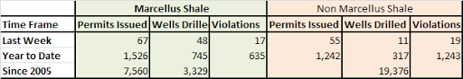
I am often asked how many Marcellus Shale wells or permits there are in Pennsylvania at the moment. The answers to these queries are growing all the time, and while I try to keep these datasets current on our DataTool to allow for mapping, the quickest way to find these answers is to look on the Well Permit Workload Report at the DEP website. The workload report is updated weekly, and has a variety of information about drilling and inspection activities over a variety of time frames. Many of the basic figures that people want to know about the industry in Pennsylvania are readily available:
Data Available on Weekly Workload Report for week ending 6-17-2011
Marcellus Shale Permit Applications
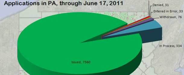
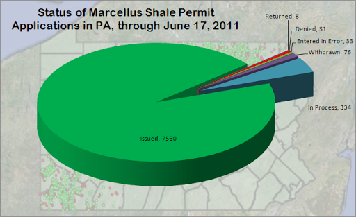
Another feature of the workload report is that it breaks down the status of Marcellus Shale permit applications from 2005 through the present.
Status of Marcellus Shale Applications in Pennsylvania, as of June 17, 2011
How selective is the process? Of the permit applications received so far, 94 percent have been approved, and four percent are still in the process of being evaluated. Only 31 applications (0.4 percent) were actually denied.
Between the Marcellus Shale and other formations, the DEP has issued over 16 permits for new wells every calendar day so far in 2011.
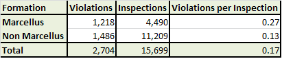
Violations per Inspection
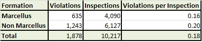
2011 year to date inspection and violation data for Pennsylvania
So far this year, non Marcellus Shale wells are slightly more likely to be issued a violation upon inspection than their Marcellus Shale counterparts. This is actually a fairly dramatic change from 2010 data, which is summarized below:
2010 inspection and violation data for Pennsylvania
Last year, there were more than twice as many violations per inspection from the Marcellus Shale than from other formations, while this year the non Marcellus wells are being flagged more often. This is both because the rate of violations per inspection for non Marcellus Shale wells has risen by 35 percent over last year’s figure, and because Marcellus Shale wells are being flagged 41 percent less often this year than last year.
One of the biggest concerns about the Marcellus Shale industry in Pennsylvania is how to deal with all of the waste products that are created in the drilling, stimulation, and production of the wells. There are also more than 40,000 oil and gas wells from other formations in the Commonwealth that reported waste production to the Pennsylvania Department of Environmental Protection (DEP) last year. Whether this waste ultimately found itself into publicly owned treatment works, industrial waste treatment facilities, injection wells, or spread on roadways, it almost always has to be shipped to a different location, sometimes hundreds of miles away.
For more information on specific facilities that accepted non Marcellus waste in 2010, click on one of the maps below, then use our information tool (“i” icon) and click on any map icon.
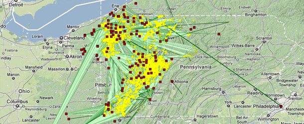
Brine
Yellow dots indicate wells that reported brine production, and red squares are receiving facilities. The green lines are the paths that the waste takes, as the crow flies. Darker lines indicate larger quantities of brine, which are measured in barrels. For more information on specific features, please click the map for a zoomable, dynamic view.
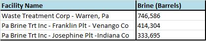
Statewide, almost 4.5 million barrels of brine was produced by non Marcellus Shale wells in 2010, which was transported over 900,000 miles as the crow flies(1) from the various wells to the facility locations, with an average one way trip of about 30 miles.
Facilities accepting the most brine from non Marcellus wells in PA in 2010
Drill Cuttings
Only one operator reported drill cutting waste from a total of three wells. All of this type of waste went to the same facility. Geographic coordinates were not included for the receiving facility in the data, so mapping and distance measurements were not performed for this analysis. Suffice it to say, however, that the amounts discussed are relatively small compared to brine and other types of waste.
Facility accepting drill cutting waste from non Marcellus wells in PA in 2010
Drilling Fluid
The color scheme for this map similar to that of brine, above, but in this view, yellow dots indicate wells producing drilling fluid waste.
More than 300,000 barrels of drilling fluid was produced last year from non Marcellus Shale wells in Pennsylvania. That waste traveled over 18,500 miles as the crow flies en route to its receiving facilities.
Facilities accepting the most drilling fluid from non Marcellus wells in PA in 2010
Frac Fluid
The color scheme for this map similar to that of brine, above, but in this view, yellow dots indicate wells producing frac fluid waste.
While the term “frac fluid” is often used to refer to the chemical additives that are used along with water and sand to hydraulically fracture a well, in terms of the waste report, it refers to the flowback water. This type of waste contains the other type of frac fluid, but at significantly reduced quantities.
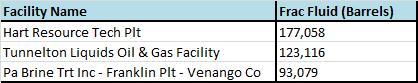
Last year, non Marcellus Shale wells reported producing over 499,000 barrels of frac fluid waste, which traveled almost 82,000 linear miles to receiving facilities, with the average one way trip being about 40 miles in length.
Facilities accepting the most frac fluid waste from non Marcellus wells ion PA in 2010
Please note, for each distance analysis, only wells from the waste production report which included decimal degree data for both the wells and receiving facilities were included. Therefore, the distances are being understated. For example, only about 29,500 of the more than 40,500 non Marcellus wells that produced brine last year are included in this figure, or about 73 percent.
https://www.fractracker.org/a5ej20sjfwe/wp-content/uploads/2011/06/Feature_2011_0616.jpg250610Matt Kelso, BAhttps://www.fractracker.org/a5ej20sjfwe/wp-content/uploads/2025/09/2025-Wordmark-Logo.pngMatt Kelso, BA2011-06-16 15:33:002020-07-21 10:38:16Movement of Pennsylvania’s non Marcellus Waste 2010
This page has been archived. It is provided for historical reference only.
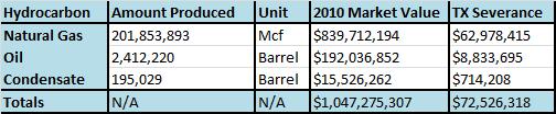
The prolific oil and gas producing state of Texas imposes a 7.5 percent severance tax on natural gas produced within the state, and 4.6 percent levies on both oil and condensate. In a recent post, I mentioned that if Pennsylvania had the same severance tax as Texas, the Commonwealth would have raised about $72.5 million last year–just from non Marcellus Shale oil and gas wells.
Estimated market value and hypothetical severance tax of non Marcellus Shale well production in 2010.
That may not be enough to plug the gaping hole in Pennsylvania’s budget, but it would at least be enough to fill a few potholes. But what if we took Marcellus Shale production into consideration as well?
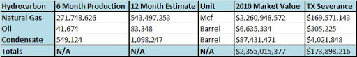
Unlike wells from other formations where the production report coincides with the calendar year, Marcellus Shale production is available for the period from July 2009 through June 2010, and from July to December 2010. While there were certainly more Marcellus wells toward the end of the year than the beginning, this is more than made up for by the likelihood that the self-reported Marcellus production data is dramatically understated. I say this because there are only 1,255 wells reporting any production in the last half of the year, and yet there were 2,498 Marcellus wells by year’s end. So while I will multiply the six month totals by two to represent the whole year, multiplying by four might be more accurate still.
Estimated market value and hypothetical severance tax of Marcellus Shale well production in 2010.
Taking the self reported data at face value, we are now looking at a hypothetical severance tax of $246 million for all formations. While that won’t solve the budget problems either, it would be enough to preserve the jobs of thousands of teachers throughout the Commonwealth.
Former Governor Rendell did little to promote a severance tax in his tenure until the very end, and Governor Corbett has stated his opposition repeatedly. However, in the interest of paying our bills without jeopardizing our fragile economic recovery, the idea of the severance tax is clearly worth another look.
It can’t be that bad for the industry. After all, they’re still drilling wells in Texas.
https://www.fractracker.org/a5ej20sjfwe/wp-content/uploads/2025/09/2025-Wordmark-Logo.png00Matt Kelso, BAhttps://www.fractracker.org/a5ej20sjfwe/wp-content/uploads/2025/09/2025-Wordmark-Logo.pngMatt Kelso, BA2011-06-10 16:08:002020-07-21 10:38:16What if Pennsylvania Had the Same Severance Tax as Texas?
This page has been archived. It is provided for historical reference only.
Oil and gas service roads in the Allegheny National Forest. Photo from the Allegheny Defense Project
The Pennsylvania Department of Environmental Protection (DEP) has recently released 2010 production and waste data for non Marcellus Shale wells. The following datasets have been added to FracTracker’s DataTool (links removed – no longer active):
PA Non Marcellus Production by Well, 2010
PA Non Marcellus Brine Production by Well, 2010
PA Non Marcellus Drill Cuttings Production by Well, 2010
PA Non Marcellus Drilling Fluid Production by Well, 2010
PA Non Marcellus Frac Fluid Production by Well, 2010
All data is self-reported by the drilling operators to the DEP.
Gas, Oil, and Condensate Production
Non-Marcellus Shale wells in Pennsylvania reported production of gas, oil, and condensate in 2010. Gas is reported in thousands of cubic feet (Mcf), while production values for oil and condensate are reported in barrels.
Natural Gas
Natural gas production in the state is significant, even without the prodigious Marcellus Shale formation that dominates current drilling activity.
2010 gas production summary in Pennsylvania for non Marcellus Shale wells
Production values vary widely throughout Pennsylvania, which of course feeds into how much royalty a landowner could make off a well on his or her property. Based on the $4.16 average wellhead price of gas for 2010, a well would have needed to produce about 1,924 Mcf of gas in order to collect $1,000, assuming the minimum one eighth share required by Pennsylvania. 36,062 of the producing wells in Pennsylvania produced that amount or less, and 28,616 earned more than that figure. The most productive non Marcellus Shale well produced 1,049,000 Mcf, which would produed a royalty check of over $540,000. The least productive wells would not qualify for any royalty check.
Vertical and horizontal non Marcellus gas well summaries and market estimates
There are some non Marcellus gas wells that are drilled horizontally now, and they are on average five times more productive than their vertical counterparts, although the sample size is fairly small. The last column, “TX Severance” calculates the estimated severance tax that would have been collected on the gas produced from Pennsylvania’s non Marcellus Shale wells, if the Commonwealth had the same 7.5 percent severance tax as Texas.
135 of 256 operators with just one well reported exactly 100 Mcf produced in 2010.
Since there is no severance tax in Pennsylvania, the most important reason to get production values correct is to make sure the landowner gets the proper royalty check. However, there are a 2,617 wells that are identified as home wells, and for these wells, royalty payments wouldn’t apply either, since the operator and the resident are the same person. Many of these wells are unmetered, according to the notes in the dataset. This probably explains why a large number of operators with just one well reported exactly 100 Mcf.
Oil and Condensate
Non Marcellus Shale wells in Pennsylvania also produced oil and condensate. Condensate is a hydrocarbon liquid or gas (depending on conditions) that is often associated with “wet gas” wells. Through the control of temperature and pressure, this is turned into liquid, removed from the natural gas stream, and sold to oil refineries. Although counted separately, condensate is fundamentally similar to light crude oil, and it is relatively easy to process into gasoline and other fuels. The average price per barrel for petroleum and other liquids in 2010 was $79.61.
Production summaries and market estimates for oil and condensate from non Marcellus Shale wells in Pennsylvania in 2010.
If Pennsylvania had the same 4.6 percent severance tax as Texas, we would have collected about $9.5 million in revenues. Combined with hypothetical gas revenues discussed above, Pennsylvania would have a handy $72.5 million to help fill in the budget gaps, just from the non Marcellus Shale wells.
Waste Production
There are five categories of waste production in the 2010 report:
Basic Sediment
Brine
Drill Cuttings
Drilling (Fluid)
Frac Fluid
Basic Sediment. This is composed of salt and other impurities that often settle at the bottom of the tank. No basic sediment was reported in Pennsylvania for non Marcellus Shale wells in 2010.
Brine. I contacted the DEP in February to clear up a point about brine for Marcellus wells. The amount of brine and frac fluid were nearly the same. Usually, “frac fluid” refers to the 1% or so of chemical fluids that are added to the sand and millions of gallons of water in order to hydraulically fracture oil and gas wells. Brine is usually one of several terms that describe this mixture once it flows back up to the surface after fracturing, having acquired significant salinity along the way. I was told that in this case, brine referred to natural underground salty waters that were encountered in the drilling process, and that frac fluid was the flow back water after fracturing operations had begun. On the other hand, I have spoken with reporters who have learned from industry sources that they treat the distinction differently: flow back water in the first 30 days are so are considered “frac fluid”, and anything thereafter is “brine”.
Regardless of how the distinction is used in practice, both are wastewater types that are difficult to dispose of. There is a movement in the industry to recycle as much as possible of these fluids for future wells. In April, the DEP asked drillers to stop disposing of these fluids in treatment plants that ultimately put the diluted fluid back into our rivers and streams. Recently, some progress has been made in those regards. Another common disposal method is the use of underground injection wells.
40,731 non Marcellus wells reported brine wastewater production in Pennsylvania in 2010, with amounts ranging from 0 to 105,000 barrels. 33,153 wells (81 percent) reported amounts of 100 barrels or less. Statewide, 4,452,905 barrels of brine were reported in 2010 for non Marcellus Shale wells, or about 187 million gallons.
Drill Cutting. Of the thousands of non Marcellus Shale wells drilled last year, apparently only one company encountered drill cuttings. Newfield Appalachia PA, LLC reported three Wayne County wells that created this type of waste that is created when the drill bit chews up thousands of feet of subterranean rock and sediment en route to the target formation. There is no word on how the other companies avoided creating drill cuttings, but in my opinion, Newfield deserves some praise for taking their reporting obligations seriously. Drill cutting waste ranged from 25 tons to 506 tons, with two wells (67 percent) reporting less than 100 tons.
Drilling Fluid. According to OSHA, there are several functions for drilling fluid, including maintaining a proper well pressure, keeping the drill bit cool, removing the drill cuttings, and preventing a collapse of the well before it has been cased. 836 wells reported drilling fluid waste, 580 of which (69 percent)reported values of under 100 barrels. The largest quantity was 45,360 barrels, an amount large enough to possibly include drill cuttings as well.
Frac Fluid For more information, see the comments for brine, above. 2,805 wells reported frac fluid waste produciton, with quantities ranging from 0 to 54,600 barrels. 2,330 wells (83 percent) reported production of less than 100 barrels of frac fluid. Statewide, there were 499,351 barrels reported, or about 22.9 million gallons.
https://www.fractracker.org/a5ej20sjfwe/wp-content/uploads/2025/09/2025-Wordmark-Logo.png00Matt Kelso, BAhttps://www.fractracker.org/a5ej20sjfwe/wp-content/uploads/2025/09/2025-Wordmark-Logo.pngMatt Kelso, BA2011-06-10 12:37:002020-07-21 10:38:16PA Non Marcellus Oil and Gas Well Data Available for 2010
by David Slottje, JD and Helen Holden Slottje, JD – Community Environmental Defense Council, Inc.
What comes to mind when you think about upstate New York? Rolling farmlands, fresh air, and the chirping of birds? Or heavy truck traffic at all hours of the day and night, the smell of chemicals in the air, distant views pockmarked with drilling rigs, and the stars blocked from sight by light pollution?
Many community groups and municipal leaders are becoming increasingly alarmed by the threats attendant to unconventional gas drilling. These communities are growing frustrated with what they perceive to be the unwillingness of state and federal politicians and agencies to act decisively. Can anything be done at the local level to protect the health and welfare of our communities? The answer is yes, at least in New York.
We are lawyers with the Community Environmental Defense Council, Inc., a pro bono, public interest environmental law firm based in Ithaca. It is our opinion that a New York municipality has the legal authority and right to use land-use laws of general applicability (such as zoning laws) to prohibit what we have termed “high-impact industrial uses,” either in certain zoning districts or throughout an entire town.
Furthermore, we believe this authority and power legally may be exercised in a manner that, depending upon the municipality’s particular definition of “high-impact industrial uses,” will have the incidental effect of prohibiting (within the town) land uses such as unconventional gas drilling.
Some people have heard that municipalities are legally restricted from enacting laws to prohibit certain uses, such as “adult entertainment,” and so they wonder whether those same restrictions might also apply to banning industrial uses. They do not.
Those restrictions on “adult entertainment” are very limited and very specific in nature, and have to do with protection of constitutional rights, specifically First Amendment rights, including free speech.
There is no question that exclusion of industrial uses is a proper and legitimate use of land-use laws.
The United States Supreme Court addressed this question in a 1974 case known as Village of Belle Terre. In Belle Terre, the court stated that the town had wide latitude to use its zoning laws to protect the public welfare, and that the public welfare is spiritual, as well as physical, aesthetic and monetary. The court specifically held that a town may use its police power “to lay out zones where the blessings of quiet seclusion and clean air make the area a sanctuary for people.”
And the New York Court of Appeals — the highest court of New York State — came to the same conclusion in a 1996 case called Gernatt Asphalt Products. This was a situation in which a town had used its zoning power to ban mining as a permitted use, and the people who wanted to mine challenged the ban, saying that the ban involved unconstitutional exclusionary zoning.
We have never held that the exclusionary zoning test, which is intended to prevent a municipality from improperly using the zoning power to keep people out, also applies to prevent the exclusion of industrial uses. […] A municipality is not obligated to permit the exploitation of any and all natural resources within the town as a permitted use, if limiting that use is a reasonable exercise of its police power to prevent damage to the rights of others and to promote the interests of the community as a whole. (Emphasis added.)
So, there should be no doubt that a New York State municipality has the legal right to use land-use laws to ban industrial uses.
You may have heard the opinion that New York has preempted the right of municipalities to ban certain specifically articulated industrial uses — oil and gas drilling and solution mining — within their boundaries.
We believe that the state has not preempted such activities, so long as they happen to fall within the definition of “high-impact industrial uses” contained in a town’s properly enacted zoning law.
There is a state statute (the “drilling statute”) that precludes municipalities from regulating the oil, gas, and solution mining industries, but we believe “regulating” means regulating the operational processes of the industry—that is, things such as how deep they can drill or mine, and imposition of bonding requirements. Municipalities may, in fact, prohibit such industries outright, either in certain zoning districts or throughout an entire town.
The drilling statute language regarding regulation is almost identical to the language regarding regulation that was previously used in the context of the mineral mining statute, and in that context the Court of Appeals made it crystal clear that the scope of preempted regulation meant regulation related to operational processes, and that municipalities absolutely could prohibit mining outright, whether in certain zoning districts or throughout an entire town.
Simply put, our recommendation to New York State municipalities seeking to preserve their character and avoid industrialization is to adopt a zoning law or amendment that specifically prohibits high-impact industrial uses within the municipality, and to utilize a definition of “high-impact industrial use” which encompasses unconventional gas drilling and any other uses determined to be inimical to the municipality’s desired character and goals.
We do not believe that our interpretation is particularly bold, or visionary, or out-of-the box. Embracing our approach does not involve attempting to create new law, or attempting to overturn any law, or even trying to distinguish a holding in an unfavorable judicial decision.
There are people out there who do not agree with our approach. Our view is that the vast majority of them are people who have a financial stake in seeing drilling go forward: drilling companies and their lawyers, landowners who favor drilling, and their lawyers—many of whom will receive substantial fees if drilling is allowed to proceed.
We would be happy to speak with the representatives of any municipality, or any community group, who wish to discuss the concepts we are recommending, the specifics of creating the type of law we are suggesting, or how to minimize political and legal “push-back” risks. We are pro bono attorneys, which means we do not charge for our time.
David Slottje is executive director and senior attorney, and Helen Holden Slottje is managing attorney, at the Community Environmental Defense Council, Inc. (CEDC). Both are members of the Club’s Atlantic Chapter. CEDC is a 501(c)(3) non-profit, pro bono, public interest environmental law firm. For more information about CEDC or to contact the authors, visit CEDC’s web site.
Copyright SierraClub 2009
https://www.fractracker.org/a5ej20sjfwe/wp-content/uploads/2025/09/2025-Wordmark-Logo.png00Guest Authorhttps://www.fractracker.org/a5ej20sjfwe/wp-content/uploads/2025/09/2025-Wordmark-Logo.pngGuest Author2011-06-07 10:46:002020-07-21 10:38:15A legal plan to control drilling
WATKINS GLEN, NY – A lawsuit by New York Attorney General Eric T. Schneiderman toforce the federal government to conduct a full environmental impact study of natural gasdrilling is a recognition of the considerable risks posed by hydraulic fracking, say membersof the grassroots Coalition to Protect New York.
“It’s regrettable that our attorney general has to go to court to force the federal governmentto do what it’s required to do under current law – protect the health and safety of itscitizens,” said Jack Ossont, spokesman for CPNY, which opposes the destructive process offracking. “We have no doubt that any rational, independent analysis of fracking will clearlyshow that the dangers far outweigh any short-term economic gains, which will benefit onlya very few anyway.”
Yesterday, Schneiderman filed a lawsuit against the federal government for its failure tocommit to a full environmental review of proposed regulations that would allow drillingfor shale gas – including the harmful technique known as fracking – in the Delaware RiverBasin.
The National Environmental Policy Act requires federal agencies to conduct a full reviewof actions that may cause significant environmental impacts. But, ignoring this law, theDelaware River Basin Commission– with the approval of its supporting federal agenciesincluding the US Army Corps of Engineers and the Environmental Protection Agency –proposed regulations allowing gas development in the Basin without undertaking any suchreview.
The proposed regulations allow high-volume hydraulic fracturing combined withhorizontal drilling (fracking) within the Basin. Fracking has been proven to pose graverisks to the environment, health, and communities. It involves the withdrawal of largevolumes of water from creeks and streams, frequent contamination of drinking watersupplies, the generation of millions of gallons of toxic waste that has to go somewhere,increased noise, dust and air pollution, and potential harms to community infrastructureand character from increased industrial activity.
“We want to thank the attorney general and all the groups involved in this matter, for pushing for an environmental impact study on fracking that should have beendone long ago,” said Ossont.
Kevin Bunger, a member of CPNY, said the attorney general’s lawsuit should allow for a full,independent, peer-reviewed study of the impacts of fracking.
“It’s irresponsible that we’ve allowed fracking to take place throughout the Northeastwithout any non-industry-funded, comprehensive analysis of its impacts on theenvironment and human health,” he said. “Of course, it hasn’t been done because a multi-state, multi-institutional, large-scale study would prove what we already know from avast array of evidence: that fracking contaminates drinking water and leads to wide-scale,probably irreversible pollution.”
CPNY members’ awareness of the destructive effects of fracking is also behind the group’sopposition to a landmark water withdrawal bill (S3798) now under consideration inthe state senate that would give away billions of gallons of New York’s waters to largeindustrial users, including the methane gas industry which requires vast amounts of waterfor its fracking operations. The assembly has already passed its version of the bill.
“There is considerable pressure on our elected officials to open our state to widespread,unregulated fracking,” said Ossont. “It’s up to the citizens of New York to tell our senatorsand representatives to do the right thing: stop and consider all the impacts. We’re beingtold that the methane gas beneath our feet presents a golden opportunity for our state andour country. But it’s fool’s gold. Fracking would ruin our environment and literally destroyour way of life.”
Contact: Jack Ossont, Coalition to Protect New York, (607) 243-7262
Left: Cabin Run orphaned oil well, Morgan County, Ohio. Many of the older oil and gas wells were either perfunctorily plugged, or else not at all. Right: The Pennsylvania DEP thinks this Bradford Township explosion in McKean County, PA might have been due to a nearby abandoned gas well that was drilled in 1881.
In April of 2000, the Pennsylvania Department of Environmental Protection (DEP) released a plan for dealing with the approximately 8,000 abandoned and orphaned oil and gas wells throughout the Commonwealth. This report singled out 550 wells that were especially problematic, and of those, 129 were flagged as the highest priority, with a point score of 30 or greater on their internal scale.
Eleven years later, there are over 8,500 abandoned and orphaned wells, and 186 with a point score of 30 or greater. Most likely, this increase doesn’t suggest newly abandoned wells so much as the discovery of additional old ones. After all, according to Independant Petroleum Association of America estimates, over 325,000 oil and gas wells were drilled statewide between 1859 and 2000. The DEP has no information on more than half of those wells–about 184,000. Therefore, the actual number of abandoned and orphaned wells in Pennsylvania could be much higher than the estimates provided above.
Abandoned wells are those that have been out of production for a year or more, and orphaned wells are wells that were abandoned prior to 1985, and from which the current landholder or operator didn’t receive any economic benefits. When wells are designated as orphaned, the DEP is responsible for plugging them. As of February, there are 6,251 wells classified as orphaned and 2,272 abandoned wells.
Reasons for Concern
Obviously, the prospects of houses suddenly exploding, as in the picture above, is reason enough to be concerned, and yet there are a variety of ways in which abandoned oil and gas wells can impact Pennsylvania’s environment and the health and well being of our residents. Most unplugged wells release some amount of oil, gas, condensate, or brine, which can kill vegetation, damage fragile riparian ecosystems, and contaminate aquifers. There is also the possibility of injury due to the sudden release of pressure. Some abandoned wells are 30 inch diameter open holes that are obviously a danger for children to fall into.
May 30, 2011 sinkhole in Allentown, PA
There is also the possibility that the presence of wells, whether active or or not, will aggravate unstable geologic formations, which are fairly common in Pennsylvania, due to mining activities in the west and soluble limestone formations in the east. This recent Allentown sinkhole was reportedly caused by a water leak, and caused significant property damage.
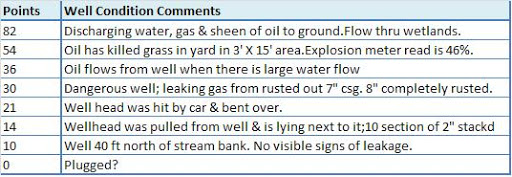
To give an example of the potential impact of abandoned oil and gas wells, here are some of the comments from the Abandoned and Orphaned Wells Program, with corresponding point scores:
Comments on abandoned wells and their corresponding point scores.
It is not always clear why a well was given a particular priority rating. Indeed, there are many instances where ratings are zero, but the comments give reason for concern, such as “Oil in water supply” and “Well intact, near implement dealer facility, is a fire hazard.” Additionally, less than 15 percent of the abandoned wells listed give any comment at all.
Incidents in McKean County
Recent explosion incidents in McKean County, PA. Please click on the gray compass rose and double chevron to hide those menus.
The Bradford Township fire mentioned above (the more southern of the two), is about half a mile from the nearest abandoned well on the list. However, the suspected well, Rogers 9, was apparently only 300 feet away. Presumably, this well was not known about until the incident occurred. Rogers 9 was drilled in 1881.
The other incident, in Foster Township, is at the northern edge of a tight cluster of recent drilling activity. It is entirely possible that there are abandoned wells in that region too, but again, nothing is on our list in the immediate vicinity.
This information leads one to suspect that one of the fires was probably due to recent activity, while the other was caused by a long-forgotten well. Whether or not that was the case, it is clear that drilling holes in the earth near where people live can have an adverse effect for a very long time.
Well Plugging
While well plugging technology has obviously improved over the years, that doesn’t necessarily mean that it is always done right. A single $25,000 bond currently is the only insurance that an operator will plug all of their wells statewide, once they are no longer in production. In most cases, that is probably adequate, since there are non-monetary incentives for the operator to stay in good graces with the DEP. However, there are numerous smaller operators with wells still in production, including some residents who have their own private wells.
In these cases, the carrot of getting the bond money returned may not match the cost of plugging the well properly, especially if multiple wells are involved. In this 1998 document, the DEP put the average cost of plugging a well between $6,000 and $22,000. Last year, the DEP plugged 11 wells in Erie County for a cost of $137,348, or a cost of about $12,500 each.
According to the Bradford Era, over 2,700 wells have already been plugged statewide under the program. In McKean County, more than 950 wells have been plugged since 1989, at a cost of over $6.5 million.
As mentioned above, the DEP assumes responsibility for plugging the orphaned wells. The money for this comes from $150 fees added to oil permit applications, and $250 fees for gas permits. Money is clearly a limiting factor in how many wells the DEP can to plug. Those 11 Erie County wells required funds from 550 new gas permits. If those wells represent the average current price for plugging a well, then the 6,251 orphaned wells still on the list would cost over $78 million to plug, requiring the permit fees from 312,550 new wells. And that is still not including the approximately 184,000 abandoned wells that the DEP doesn’t even know about.
Maybe it is time for a new strategy.
https://www.fractracker.org/a5ej20sjfwe/wp-content/uploads/2025/09/2025-Wordmark-Logo.png00Matt Kelso, BAhttps://www.fractracker.org/a5ej20sjfwe/wp-content/uploads/2025/09/2025-Wordmark-Logo.pngMatt Kelso, BA2011-06-03 10:27:002023-03-09 13:59:54Problems with Abandoned and Orphaned Wells
Marcellus Shale violations issued by the Pennsylvania DEP from January through April, 2011.
Violation information from April was recently posted on the Department of Environmental Protection (DEP) website, and two new violations datasets have been posted on our DataTool as well, including:
As the titles indicate, these datasets contain inspection and enforcement data in addition to violations, which allow us to take a closer look at both violations per inspection and enforcements actions per violation.
Violations per Inspection
Marcellus Shale violations per inspection, 2010. For a dynamic, zoomable view, please click the map.
[map archived] Marcellus Shale violations per inspection, January through April 2011
In 2010, Marcellus Shale wells in the northeastern portion of the state had a noticeably higher number of violations per inspection than the southwest. This trend is less pronounced so far in 2011. I should point out that since each inspection on this report lead to at least one violation, it is more accurate to think of this category as “violations per inspection yielding violations”, a cumbersome but significant distinction.
Enforcements per Violation
Marcellus Shale enforcement actions per violation, 2010
[map archived]
Marcellus Shale enforcement actions per violation, January through April, 2011
While the northeastern portion of Pennsylvania has a higher number of violations issued per inspection, the southwest has a higher number of enforcement actions, a category which includes fines and other restrictions imposed on drilling operators by the DEP. This trend seems to continue into 2011, with relatively minor changes in distribution.
https://www.fractracker.org/a5ej20sjfwe/wp-content/uploads/2025/09/2025-Wordmark-Logo.png00Matt Kelso, BAhttps://www.fractracker.org/a5ej20sjfwe/wp-content/uploads/2025/09/2025-Wordmark-Logo.pngMatt Kelso, BA2011-05-31 15:14:002020-07-21 10:37:59Marcellus Shale Violations per Inspection and Enforcements per Violation
Fire in Hopewell Township PA,
Southwestern PA on 3-31-10
Earlier this week, a Pennsylvania Senate committee approved a bill that would require natural gas drilling companies to provide emergency response information to local authorities. Here are the key requirements of drilling companies that are being proposed:
Post emergency response information at each well site
Register distinct geographic coordinates for each drilling site with the PA Department of Environmental Protection and local authorities
File response plans with the local authorities, local 911 center, PA DEP, and PA Emergency Management Agency
Inadequate data transparency of this type has been a significant public health concern ever since natural gas drilling first began in the Marcellus Shale region in PA.Marcellus Shale sites are often drilled in rural, remote areas without exact location information or clear emergency plans. If passed into law, this legislation stands to decrease the response time in the event of an emergency at a well site, reducing the impact that drilling incidents may have on public health and the environment.
To demonstrate why improving the quality and expediency of emergency response to shale gas drilling incidents is an important endeavor, below is a map created on FracTracker’s DataTool showing only the location of violations issued by the PA DEP in 2010 to companies that were drilling into the Marcellus Shale layer. If you press “Click to see more details on this map,” you can use the DataTool to filter the dataset even further in order to see which of these violations was an environmental health and safety violation, not just administrative in nature:
(Darker diamonds indicate there was more than one violation issued in that area. Zoom in to learn more.)
https://www.fractracker.org/a5ej20sjfwe/wp-content/uploads/2025/09/2025-Wordmark-Logo.png00FracTracker Alliancehttps://www.fractracker.org/a5ej20sjfwe/wp-content/uploads/2025/09/2025-Wordmark-Logo.pngFracTracker Alliance2011-05-25 18:25:002020-07-21 10:37:59Data Transparency Bill Will Aid Emergency Response
Year to date drilled wells in Pennsylvania. Click the map for a larger, dynamic view.
I have updated the 2011 drilled wells information on FracTracker’s DataTool. There are several interesting trends to point out, including:
Percentage of wells from the Marcellus Shale formation
Drilling operator trends
Non Marcellus horizontal well data
Marcellus Shale and Other Formations
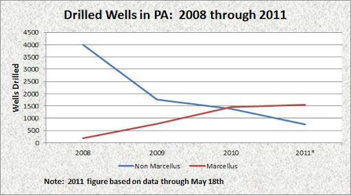
So far in 2011, 587 Marcellus Shale wells have been drilled in Pennsylvania, compared to only 281 from other formations. This means that for the first time, Marcellus wells account for over two thirds of the drilling activity statewide.
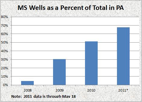
In less than three and a half years, the Marcellus Shale went from representing 5% of all oil and gas wells drilled in Pennsylvania to 68%.
Drilling trends over time in Pennsylvania.
While part of the reason for the Marcellus Shale’s increased prominence in the oil and gas industry in Pennsylvania is that activity in the formation is rapidly increasing, it is also true that activities in other formations are decreasing rather dramatically.
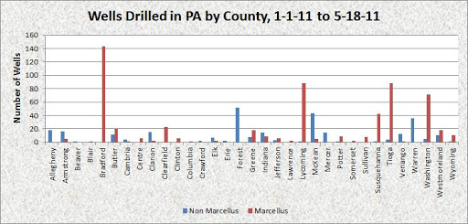
We can also take a look at drilling activity by county for both Marcellus Shale and other oil and gas wells.
Marcellus Shale and other wells drilled to date in 2011 by county.
Much of the above chart has to do with where the hydrocarbon resources are. It is interesting to note though, that the county with the most Marcellus wells (Bradford) has no wells in other formations, and that the county with the most non Marcellus wells (Forest) has no Marcellus wells at all.
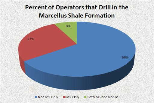
Drilling Operators and the Marcellus Shale
Of the 91 operators that have drilled oil and gas wells so far this year in Pennsylvania, 60 had no Marcellus Shale wells, 25 had only Marcellus Shale wells, and seven had wells in both categories.
Most operators drill in either the Marcellus Shale or other formations, but not both.
There is surprisingly little overlap in this chart. But what about the operators with wells in both categories?
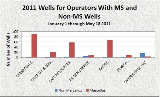
Marcellus and non Marcellus wells for operators with both categories in 2011.
Even still, most of the operators specialize in one kind or the other. Taken together, these two charts show that operators which drill in the Marcellus Shale are specialists, with very few wells drilled in other formations.
Non Marcellus Horizontal Wells
It is well known that the combination of hydraulic fracturing and horizontal drilling techniques allowed for the profitable extraction of natural gas from the Marcellus Shale. For that reason, it isn’t surprising that most of the Marcellus wells are drilled horizontally. What is interesting is that the technique is now being used in other formations as well.
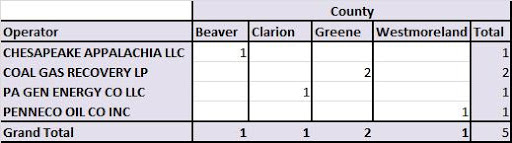
Five Non Marcellus Shale wells have been horizontally drilled so far in 2011.
Non Marcellus horizontal wells so far in 2011.
There isn’t much of a trend in which companies drilled these five wells, with two of the companies active in the Marcellus Shale and two of them not. Spatially, all four of the counties are in the western portion of the state, with Clarion County somewhat to the north of the other three.
https://www.fractracker.org/a5ej20sjfwe/wp-content/uploads/2025/09/2025-Wordmark-Logo.png00Matt Kelso, BAhttps://www.fractracker.org/a5ej20sjfwe/wp-content/uploads/2025/09/2025-Wordmark-Logo.pngMatt Kelso, BA2011-05-18 12:42:002020-07-21 10:37:59Year to Date Drilling Activity in Pennsylvania