Groundwater risks in Colorado due to Safe Drinking Water Act exemptions
Oil and gas operators are polluting groundwater in Colorado, and the state and U.S. EPA are granting them permission with exemptions from the Safe Drinking Water Act.
FracTracker Alliance’s newest analysis attempts to identify groundwater risks in Colorado groundwater from the injection of oil and gas waste. Specifically, we look at groundwater monitoring data near Class II underground injection control (UIC) disposal wells and in areas that have been granted aquifer exemptions from the underground source of drinking water rules of the Safe Drinking Water Act (SDWA). Momentum to remove amend the SDWA and remove these exemption.
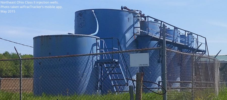
Learn more about Class II injection wells.
Aquifer exemptions are granted to allow corporations to inject hazardous wastewater into groundwater aquifers. The majority, two-thirds, of these injection wells are Class II, specifically for oil and gas wastes.
What exactly are aquifer exemptions?
The results of this assessment provide insight into high-risk issues with aquifer exemptions and Class II UIC well permitting standards in Colorado. We identify areas where aquifer exemptions have been granted in high quality groundwater formations, and where deep underground aquifers are at risk or have become contaminated from Class II disposal wells that may have failed.
Of note: On March 23, 2016, NRDC submitted a formal petition urging the EPA to repeal or amend the aquifer exemption rules to protect drinking water sources and uphold the Safe Drinking Water Act. Learn more
Research shows injection wells do fail
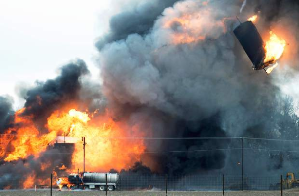
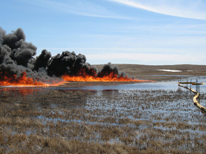
Class II injection well in Colorado explodes and catches fire. Photo by Kelsey Brunner for the Greeley Tribune.
Disposal of oil and gas wastewater by underground injection has not yet been specifically researched as a source of systemic groundwater contamination nationally or on a state level. Regardless, this issue is particularly pertinent to Colorado, since there are about 3,300 aquifer exemptions in the US (view map), and the majority of these are located in Montana, Wyoming, and Colorado. There is both a physical risk of danger as well as the risk of groundwater contamination. The picture to the right shows an explosion of a Class II injection well in Greeley, CO, for example.
Applicable and existing research on injection wells shows that a risk of groundwater contamination of – not wastewater – but migrated methane due to a leak from an injection well was estimated to be between 0.12 percent of all the water wells in the Colorado region, and was measured at 4.5 percent of the water wells that were tested in the study.
A recent article by ProPublica quoted Mario Salazar, an engineer who worked for 25 years as a technical expert with the EPA’s underground injection program in Washington:
In 10 to 100 years we are going to find out that most of our groundwater is polluted … A lot of people are going to get sick, and a lot of people may die.
Also in the ProPublic article was a study by Abrahm Lustgarten, wherein he reviewed well records and data from more than 220,000 oil and gas well inspections, and found:
- Structural failures inside injection wells are routine.
- Between 2007-2010, one in six injection wells received a well integrity violation.
- More than 7,000 production and injection wells showed signs of well casing failures and leakage.
This means disposal wells can and do fail regularly, putting groundwater at risk. According to Chester Rail, noted groundwater contamination textbook author:
…groundwater contamination problems related to the subsurface disposal of liquid wastes by deep-well injection have been reviewed in the literature since 1950 (Morganwalp, 1993) and groundwater contamination accordingly is a serious problem.
According to his textbook, a 1974 U.S. EPA report specifically warns of the risk of corrosion by oil and gas waste brines on handling equipment and within the wells. The potential effects of injection wells on groundwater can even be reviewed in the U.S. EPA publications (1976, 1996, 1997).
As early as 1969, researchers Evans and Bradford, who reported on the dangers that could occur from earthquakes on injection wells near Denver in 1966, had warned that deep well injection techniques offered temporary and not long-term safety from the permanent toxic wastes injected.
Will existing Class II wells fail?
For those that might consider data and literature on wells from the 1960’s as being unrepresentative of activities occurring today, of the 587 wells reported by the Colorado’s oil and gas regulatory body, COGCC, as “injecting,” 161 of those wells were drilled prior to 1980. And 104 were drilled prior to 1960!
Wells drilled prior to 1980 are most likely to use engineering standards that result in “single-point-of-failure” well casings. As outlined in the recent report from researchers at Harvard on underground natural gas storage wells, these single-point-of-failure wells are at a higher risk of leaking.
It is also important to note that the U.S. EPA reports only 569 injection wells for Colorado, 373 of which may be disposal wells. This is a discrepancy from the number of injection wells reported by the COGCC.
Aquifer Exemptions in Colorado
According to COGCC, prior to granting a permit for a Class II injection well, an aquifer exemption is required if the aquifer’s groundwater test shows total dissolved solids (TDS) is between 3,000 and 10,000 milligrams per liter (mg/l). For those aquifer exemptions that are simply deeper than the majority of current groundwater wells, the right conditions, such as drought, or the needs of the future may require drilling deeper or treating high TDS waters for drinking and irrigation. How the state of Colorado or the U.S. EPA accounts for economic viability is therefore ill-conceived.
Data Note: The data for the following analysis came by way of FOIA request by Clean Water Action focused on the aquifer exemption permitting process. The FOIA returned additional data not reported by the US EPA in the public dataset. That dataset contained target formation sampling data that included TDS values. The FOIA documents were attached to the EPA dataset using GIS techniques. These GIS files can be found for download in the link at the bottom of this page.
Map 1. Aquifer exemptions in Colorado
View map fullscreen | How FracTracker maps work
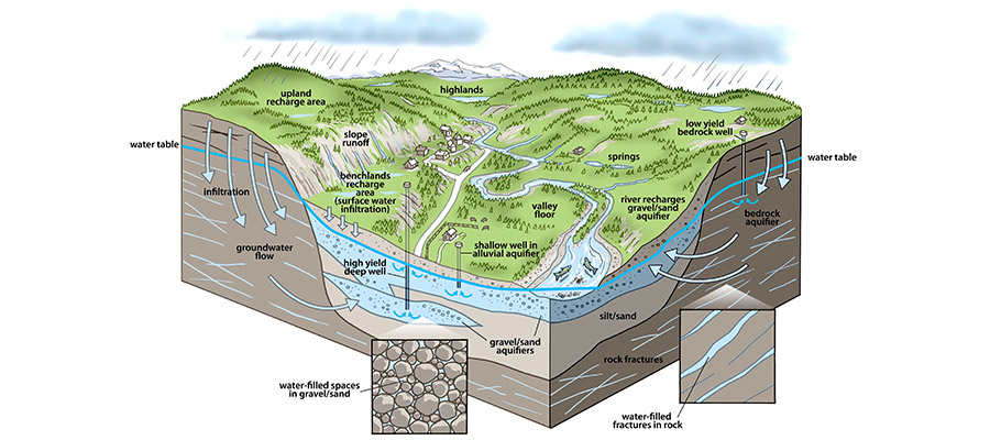
Map 1 above shows the locations of aquifer exemptions in Colorado, as well as the locations of Class II injection wells. These sites are overlaid on a spatial assessment of groundwater quality (a map of the groundwater’s quality), which was generated for the entire state. The changing colors on the map’s background show spatial trends of TDS values, a general indicator of overall groundwater quality.
In Map 1 above, we see that the majority of Class II injection wells and aquifer exemptions are located in regions with higher quality water. This is a common trend across the state, and needs to be addressed.
Our review of aquifer exemption data in Colorado shows that aquifer exemption applications were granted for areas reporting TDS values less than 3,000 mg/l, which contradicts the information reported by the COGCC as permitting guidelines. Additionally, of the 175 granted aquifer exemptions for which the FOIA returned data, 141 were formations with groundwater samples reported at less than 10,000 mg/l TDS. This is half of the total number (283) of aquifer exemptions in the state of Colorado.
When we mapped where class II injection wells are permitted, a total of 587 class II wells were identified in Colorado, outside of an aquifer exemption area. Of the UIC-approved injection wells identified specifically as disposal wells, at least 21 were permitted outside aquifer exemptions and were drilled into formations that were not hydrocarbon producing. Why these injection wells are allowed to operate outside of an aquifer exemption is unknown – a question for regulators.
You can see in the map that most of the aquifer exemptions and injection wells in Colorado are located in areas with lower TDS values. We then used GIS to conduct a spatial analysis that selected groundwater wells within five miles of the 21 that were permitted outside aquifer exemptions. Results show that groundwater wells near these sites had consistently low-TDS values, meaning good water quality. In Colorado, where groundwater is an important commodity for a booming agricultural industry and growing cities that need to prioritize municipal sources, permitting a Class II disposal well in areas with high quality groundwater is irresponsible.
Groundwater Monitoring Data Maps
Map 2. Water quality and depths of groundwater wells in Colorado
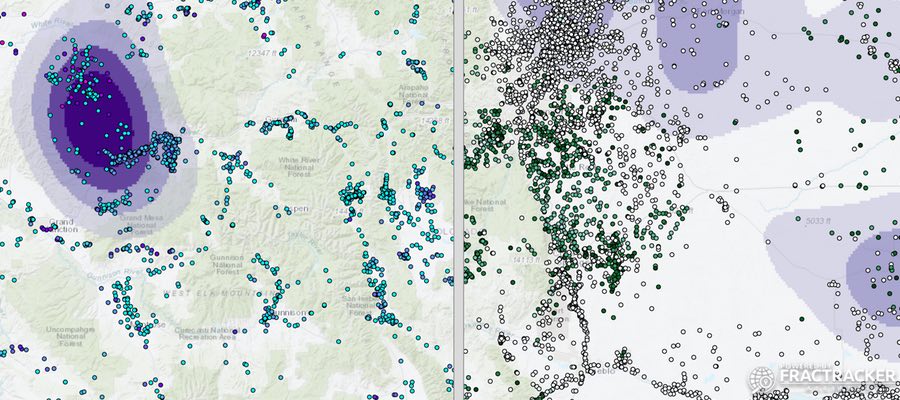
View live map | How FracTracker maps work
In Map 2, above, the locations of groundwater wells in Colorado are shown. The colors of the dots represent the concentration of TDS on the right and well depth on the left side of the screen. By sliding the bar on the map, users can visualize both. This feature allows people to explore where deep wells also are characterized by high levels of TDS. Users can also see that areas with high quality low TDS groundwater are the same areas that are the most developed with oil and gas production wells and Class II injection wells, shown in gradients of purple.
Statistical analysis of this spatial data gives a clearer picture of which regions are of particular concern; see below in Map 3.
Map 3. Spatial “hot-spot” analysis of groundwater quality and depth of groundwater wells in Colorado
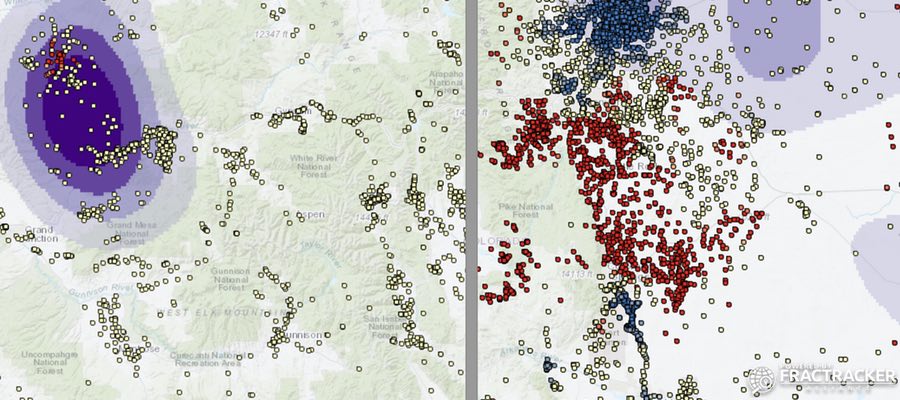
View live map | How FracTracker maps work
In Map 3, above, the data visualized in Map 2 were input into a hot-spots analysis, highlighting where high and low values of TDS and depth differ significantly from the rest of the data. The region of the Front Range near Denver has significantly deeper wells, as a result of population density and the need to drill municipal groundwater wells.
The Front Range is, therefore, a high-risk region for the development of oil and gas, particularly from Class II injection wells that are necessary to support development.
Methods Notes: The COGCC publishes groundwater monitoring data for the state of Colorado, and groundwater data is also compiled nationally by the Advisory Committee on Water Information (ACWI). (Data from the National Groundwater Monitoring Network is sponsored by the ACWI Subcommittee on Ground Water.) These datasets were cleaned, combined, revised, and queried to develop FracTracker’s dataset of Colorado groundwater wells. We cleaned the data by removing sites without coordinates. Duplicates in the data set were removed by selecting for the deepest well sample. Our dataset of water wells consisted of 5,620 wells. Depth data was reported for 3,925 wells. We combined this dataset with groundwater data exported from ACWI. Final count for total wells with TDS data was 11,754 wells. Depth data was reported for 7,984 wells. The GIS files can be downloaded in the compressed folder at the bottom of this page.
Site Assessments – Exploring Specific Regions
Particular regions were further investigated for impacts to groundwater, and to identify areas that may be at a high risk of contamination. There are numerous ways that groundwater wells can be contaminated from other underground activity, such as hydrocarbon exploration and production or waste injection and disposal. Contamination could be from hydraulic fracturing fluids, methane, other hydrocarbons, or from formation brines.
From the literature, brines and methane are the most common contaminants. This analysis focuses on potential contamination events from brines, which can be detected by measuring TDS, a general measure for the mixture of minerals, salts, metals and other ions dissolved in waters. Brines from hydrocarbon-producing formations may include heavy metals, radionuclides, and small amounts of organic matter.
Wells with high or increasing levels of TDS are a red flag for potential contamination events.
Methods
Groundwater wells at deep depths with high TDS readings are, therefore, the focus of this assessment. Using GIS methods we screened our dataset of groundwater wells to only identify those located within a buffer zone of five miles from Class II injection wells. This distance was chosen based on a conservative model for groundwater contamination events, as well as the number of returned sample groundwater wells and the time and resources necessary for analysis. We then filtered the groundwater wells dataset for high TDS values and deep well depths to assess for potential impacts that already exist. We, of course, explored the data as we explored the spatial relationships. We prioritized areas that suggested trends in high TDS readings, and then identified individual wells in these areas. The data initially visualized were the most recent sampling events. For the wells prioritized, prior sampling events were pulled from the data. The results were graphed to see how the groundwater quality has changed over time.
Case of Increasing TDS Readings
If you zoom to the southwest section of Colorado in Map 2, you can see that groundwater wells located near the injection well 1 Fasset SWD (EPA) (05-067-08397) by Operator Elm Ridge Exploration Company LLC were disproportionately high (common). Groundwater wells located near this injection well were selected for, and longitudinal TDS readings were plotted to look for trends in time. (Figure 1.)
The graphs in Figure 1, below, show a consistent increase of TDS values in wells near the injection activity. While the trends are apparent, the data is limited by low numbers of repeated samples at each well, and the majority of these groundwater wells have not been sampled in the last 10 years. With the increased use of well stimulation and enhanced oil recovery techniques over the course of the last 10 years, the volumes of injected wastewater has also increased. The impacts may, therefore, be greater than documented here.
This area deserves additional sampling and monitoring to assess whether contamination has occurred.


Figures 1a and 1b. The graphs above show increasing TDS values in samples from groundwater wells in close proximity to the 1 Fassett SWD wellsite, between the years 2004-2015. Each well is labeled with a different color. The data for the USGS well in the graph on the right was not included with the other groundwater wells due to the difference in magnitude of TDS values (it would have been off the chart).
Groundwater Contamination Case in 2007
We also uncovered a situation where a disposal well caused groundwater contamination. Well records for Class II injection wells in the southeast corner of Colorado were reviewed in response to significantly high readings of TDS values in groundwater wells surrounding the Mckinley #1-20-WD disposal well.
When the disposal well was first permitted, farmers and ranchers neighboring the well site petitioned to block the permit. Language in the grant application is shown below in Figure 2. The petitioners identified the target formation as their source of water for drinking, watering livestock, and irrigation. Regardless of this petition, the injection well was approved. Figure 3 shows the language used by the operator Energy Alliance Company (EAC) for the permit approval, which directly contradicts the information provided by the community surrounding the wellsite. Nevertheless, the Class II disposal well was approved, and failed and leaked in 2007, leading to the high TDS readings in the groundwater in this region.
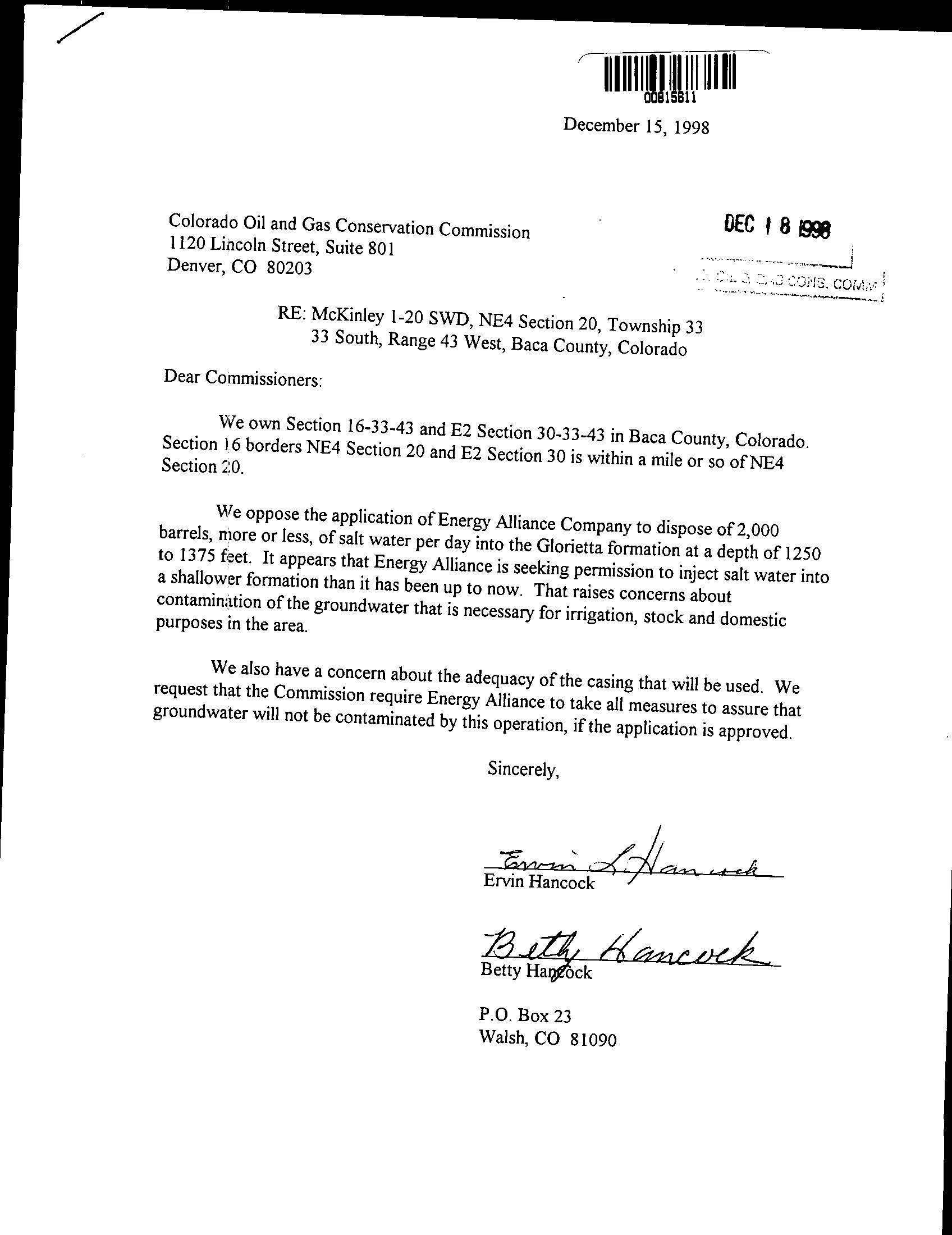
Figure 2. Petition by local landowners opposing the use of their drinking water source formation for the site of a Class II injection disposal well.
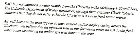
Figure 3. The oil and gas operation EAC claims the Glorietta formation is not a viable fresh water source, directly contradicting the neighboring farmers and ranchers who rely on it.
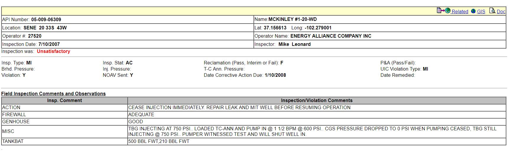
Figure 4. The COGCC well log report shows a casing failure, and as a result a leak that contaminated groundwater in the region.
Areas where lack of data restricted analyses
In other areas of Colorado, the lack of recent sampling data and longitudinal sampling schemes made it even more difficult to track potential contamination events. For these regions, FracTracker recommends more thorough sampling by the regulatory agencies COGCC and USGS. This includes much of the state, as described below.
Southeastern Colorado
Our review of the groundwater data in southeastern Colorado showed a risk of contamination considering the overlap of injection well depths with the depths of drinking water wells. Oil and gas extraction and Class II injections are permitted where the aquifers include the Raton formation, Vermejo Formation, Poison Canyon Formation and Trinidad Sandstone. Groundwater samples were taken at depths up to 2,200 ft with a TDS value of 385 mg/l. At shallower depths, TDS values in these formations reached as high as 6,000 mg/l, and 15 disposal wells are permitted in aquifer exemptions in this region. Injections in this area start at around 4,200 ft.
In Southwestern Colorado, groundwater wells in the San Jose Formation are drilled to documented depths of up to 6,000 feet with TDS values near 2,000 mg/l. Injection wells in this region begin at 565 feet, and those used specifically for disposal begin at below 5,000 feet in areas with aquifer exemptions. There are also four disposal wells outside of aquifer exemptions injecting at 5,844 feet, two of which are not injecting into active production zones at depths of 7,600 and 9,100 feet.
Western Colorado
In western Colorado well Number 1-32D VANETA (05-057-06467) by Operator Sandridge Exploration and Production LLC’s North Park Horizontal Niobara Field in the Dakota-Lokota Formation has an aquifer exemption. The sampling data from two groundwater wells to the southeast, near Coalmont, CO, were reviewed, but we can’t get a good picture due to the lack of repeat sampling.
Northwestern Colorado
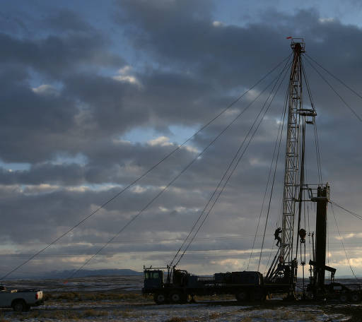
A crew from Bonanza Creek repairs an existing well in the McCallum oil field. Photo by Ken Papaleo / Rocky Mountain News
In Northwestern Colorado near Walden, CO and the McCallum oil field, two groundwater wells with TDS above 10,000 ppm were selected for review. There are 21 injection wells in the McCallum field to the northwest. Beyond the McCallum field is the Battleship field with two wastewater disposal wells with an aquifer exemption. West of Grover, Colorado, there are several wells with high TDS values reported for shallow wells. Similar trends can be seen near Vernon. The data on these wells and wells from along the northern section of the Front Range, which includes the communities of Fort Collins, Greeley, and Longmont, suffered from the same issue. Lack of deep groundwater well data coupled with the lack of repeat samples, as well as recent sampling inhibited the ability to thoroughly investigate the threat of contamination.
Trends and Future Development
Current trends in exploration and development of unconventional resources show the industry branching southwest of Weld County towards Fort Collins, Longmont, Broomfield and Boulder, CO.
These regions are more densely populated than the Front Range county of Weld, and as can be seen in the maps, the drinking water wells that access groundwaters in these regions are some of the deepest in the state.
This analysis shows where Class II injection has already contaminated groundwater resources in Colorado. The region where the contamination has occurred is not unique; the drinking water wells are not particularly deep, and the density of Class II wells is far from the highest in the state.
Well casing failures and other injection issues are not exactly predictable due to the variety of conditions that can lead to a well casing failure or blow-out scenario, but they are systemic. The result is a hazardous scenario where it is currently difficult to mitigate risk after the injection wells are drilled.
Allowing Class II wells to expand into Front Range communities that rely on deep wells for municipal supplies is irresponsible and dangerous.
The encroachment of extraction into these regions, coupled with the support of Class II injection wells to handle the wastewater, would put these groundwater wells at particular risk of contamination. Based on this analysis, we recommend that regulators take extra care to avoid permitting Class II wells in these regions as the oil and gas industry expands into new areas of the Front Range, particularly in areas with dense populations.
Feature Image: Joshua Doubek / WIKIMEDIA COMMONS
Article by: Kyle Ferrar, Western Program Coordinator, FracTracker Alliance
October 31, 2017 Edit: This post originally cited the Clean Water Act instead of the Safe Drinking Water Act as the source that EPA uses to grant aquifer exemptions.


")
")
")
")
")
")

")

")


")
")


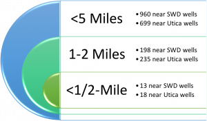 Just how close are public water supplies to Class II waste disposal wells and permitted Utica wells? As of January 15, 2017, there are 13 PWS’s within a half-mile of Ohio’s Class II SWD wells, and 18 within a half-mile of permitted Utica wells. These facilities serve approximately 2,000 Ohioans each, with an average of 112-153 people per PWS (Tables 1 and 5). Within one mile from these wells there are 64 to 66 PWSs serving 18 to 61 thousand Ohioans. That’s an average of 285-925 residents.